13.11 Replications

Little recap: There is a trade-off between type I & type II error

• Type I error reject \(H_0\) when \(H_0\) is TRUE
• Type I error Rate is the prob of type I error
• Type II error no reject \(H_0\) when \(H_0\) is FALSE
• POWER of hypothesis is the prob of not making type II error

credit: Federica Gazzelloni

• R: sum of the number of pvalues which are below the threshold and will be rejected (n. rejections)
• m: total hypothesis testing
• m0: negatives
• m1: m-m0 positives

Now what we do is replicating the sample in a lab environment to obtain fake data, in order to do that we generate a matrix from a replication of normal distribution of the same size of our data.

n <- 24
m <- 8793
delta <- 2 # this is the sample split in two
positives <- 500 # m1
# negatives
m0<- m-positives # 8293

mat <- matrix(rnorm(n*m),m,n)
mat[1:positives,1:(n/2)] <- mat[1:positives,1:(n/2)] + delta

Then we do 1000 replications to see in what is the false discovery rate for this lab.

B<-1000
set.seed(1173)
results_global <- replicate(B,{
  mat <- matrix(rnorm(n*m),m,n)
  mat[1:positives,1:(n/2)] <- mat[1:positives,1:(n/2)] + delta
  pvals = genefilter::rowttests(mat,null_hypothesis)$p.val
  ##Bonferroni
  FP1 <- sum(pvals[-(1:positives)]<=0.05/m)  
  FN1 <- sum(pvals[1:positives]>0.05/m)
  # p.adjust
  qvals1 <- p.adjust(pvals,method = "fdr")
  FP2<-sum(qvals1[-(1:positives)]<=0.05)
  FN2 <- sum(qvals1[1:positives]>0.05)
  # qvalue
  qvals2 <- qvalue::qvalue(pvals)$qvalues
  FP3<-sum(qvals2[-(1:positives)]<=0.05)
  FN3 <- sum(qvals2[1:positives]>0.05)
  c(FP1,FN1,FP2,FN2,FP3,FN3)
}) 

class(results_global)

## [1] "matrix" "array"

In this table are summarised the: false positives (FP) and the false negatives (FN) for three methods:

• Bonferroni
• FDR with p.adjust()
• FDR with qvalue()

The counts for FP and FN for the three cases:

##              V1  V2  V3  V4  V5  V6
## FP1           0   0   0   0   0   0
## FN1         383 382 372 391 383 369
## FP2-padjust  22  22  20  32  22  20
## FN2-padjust  42  29  34  28  38  30
## FP3-qvalue   24  22  20  35  24  24
## FN3-qvalue   38  28  33  27  34  29

The mean values or the proportions for the same methods:

##   id   Bonferroni FDR...padjust FDR...qvalue
## 1 FP 4.461594e-06   0.002773906  0.002960328
## 2 FN 7.645120e-01   0.081822000  0.077982000

---

Benjamini-Hochberg

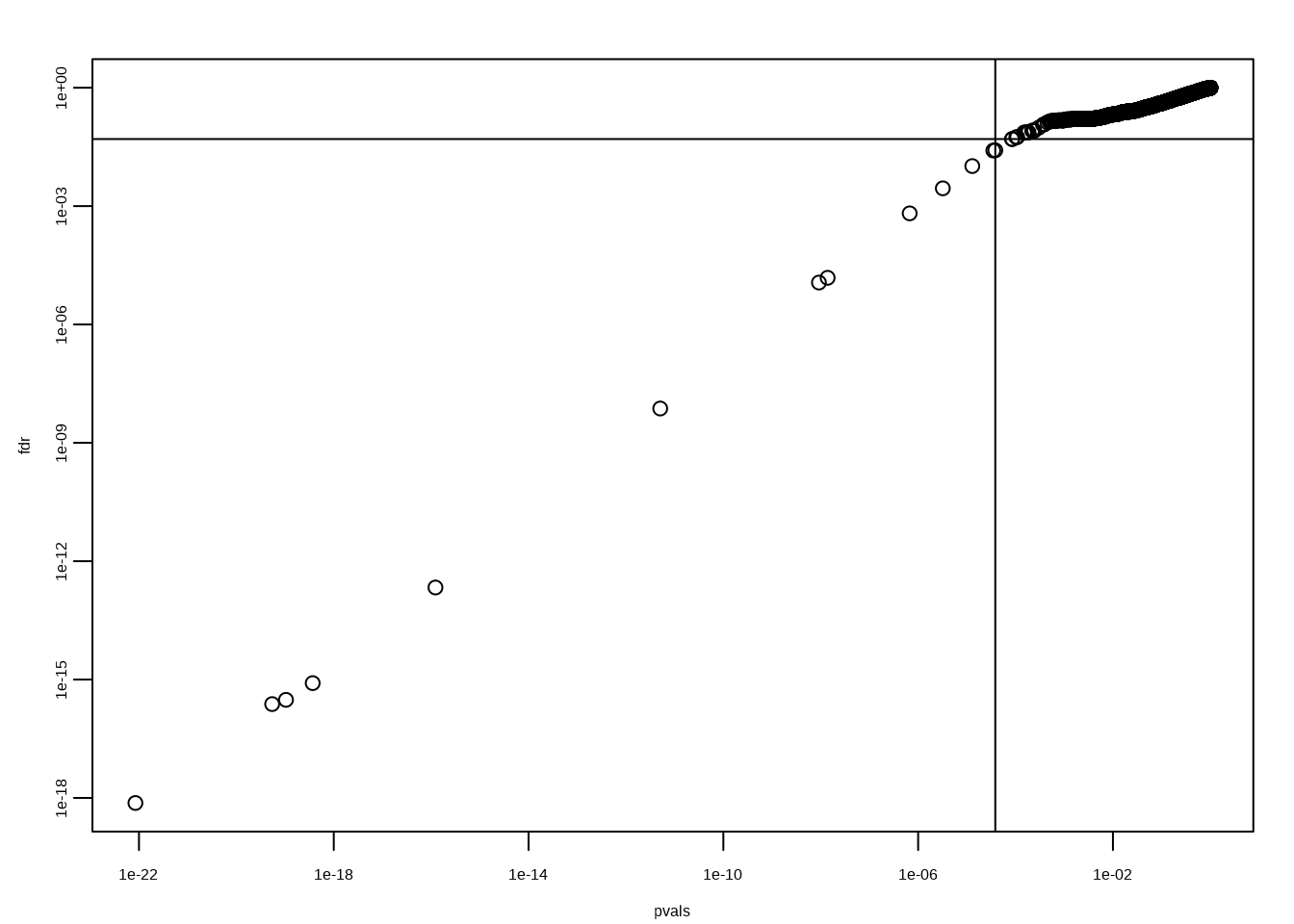
\[p(i)≤\frac{i}{m}\alpha\]

alpha <- 0.05
i = seq(along=pvals)

mypar(1,2)
plot(i,sort(pvals))
abline(0,i/m*alpha)
##close-up
plot(i[1:15],sort(pvals)[1:15],main="Close-up")
abline(0,i/m*alpha)

k <- max( which( sort(pvals) < i/m*alpha) )
cutoff <- sort(pvals)[k]
cat("k =",k,"p-value cutoff=",cutoff)

## k = 13 p-value cutoff= 3.83879e-05

fdr <- p.adjust(pvals, method="fdr")
mypar(1,1)
plot(pvals,fdr,log="xy")
abline(h=alpha,v=cutoff)

---