7.5 Applied Exercises
- For the
Wagedata
- polynomial regression
# Cross validation to choose degree of polynomial.
set.seed(1)
cv.error.10 = rep(0,10)
for (i in 1:10) {
glm.fit=glm(wage~poly(age,i),data=Wage)
cv.error.10[i]=cv.glm(Wage,glm.fit,K=10)$delta[1]
}
plot(cv.error.10, type="b", xlab="Degree", ylab="CV Error")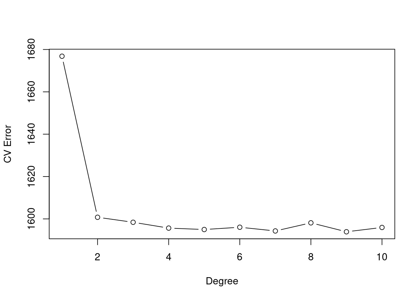
The cross-validation error seems stagnant after degree-4 use.
lm.fit = glm(wage ~ poly(age,4), data = Wage)
summary(lm.fit)
##
## Call:
## glm(formula = wage ~ poly(age, 4), data = Wage)
##
## Coefficients:
## Estimate Std. Error t value Pr(>|t|)
## (Intercept) 111.7036 0.7287 153.283 < 2e-16 ***
## poly(age, 4)1 447.0679 39.9148 11.201 < 2e-16 ***
## poly(age, 4)2 -478.3158 39.9148 -11.983 < 2e-16 ***
## poly(age, 4)3 125.5217 39.9148 3.145 0.00168 **
## poly(age, 4)4 -77.9112 39.9148 -1.952 0.05104 .
## ---
## Signif. codes: 0 '***' 0.001 '**' 0.01 '*' 0.05 '.' 0.1 ' ' 1
##
## (Dispersion parameter for gaussian family taken to be 1593.19)
##
## Null deviance: 5222086 on 2999 degrees of freedom
## Residual deviance: 4771604 on 2995 degrees of freedom
## AIC: 30641
##
## Number of Fisher Scoring iterations: 2# Using Anova() to compare degree 4 model with others.
fit.1 = lm(wage~age ,data=Wage)
fit.2 = lm(wage~poly(age ,2) ,data=Wage)
fit.3 = lm(wage~poly(age ,3) ,data=Wage)
fit.4 = lm(wage~poly(age ,4) ,data=Wage)
fit.5 = lm(wage~poly(age ,5) ,data=Wage)
anova(fit.1,fit.2,fit.3,fit.4,fit.5)## Analysis of Variance Table
##
## Model 1: wage ~ age
## Model 2: wage ~ poly(age, 2)
## Model 3: wage ~ poly(age, 3)
## Model 4: wage ~ poly(age, 4)
## Model 5: wage ~ poly(age, 5)
## Res.Df RSS Df Sum of Sq F Pr(>F)
## 1 2998 5022216
## 2 2997 4793430 1 228786 143.5931 < 2.2e-16 ***
## 3 2996 4777674 1 15756 9.8888 0.001679 **
## 4 2995 4771604 1 6070 3.8098 0.051046 .
## 5 2994 4770322 1 1283 0.8050 0.369682
## ---
## Signif. codes: 0 '***' 0.001 '**' 0.01 '*' 0.05 '.' 0.1 ' ' 1ANOVA check shows significance between models stops after degree-4.
# Grid of values for age at which we want predictions.
agelims=range(age)
age.grid=seq(from=agelims[1],to=agelims[2])
# Predictions.
preds=predict(lm.fit,newdata=list(age=age.grid),se=TRUE)
se.bands=cbind(preds$fit+2*preds$se.fit,preds$fit-2*preds$se.fit)
# Plot of polynomial fit onto data including SE bands.
plot(age,wage,xlim=agelims,cex=.5,col="darkgrey")
title("Polynomial fit using degree 4")
lines(age.grid,preds$fit,lwd=2,col="blue")
matlines(age.grid,se.bands,lwd =1,col="blue",lty =3)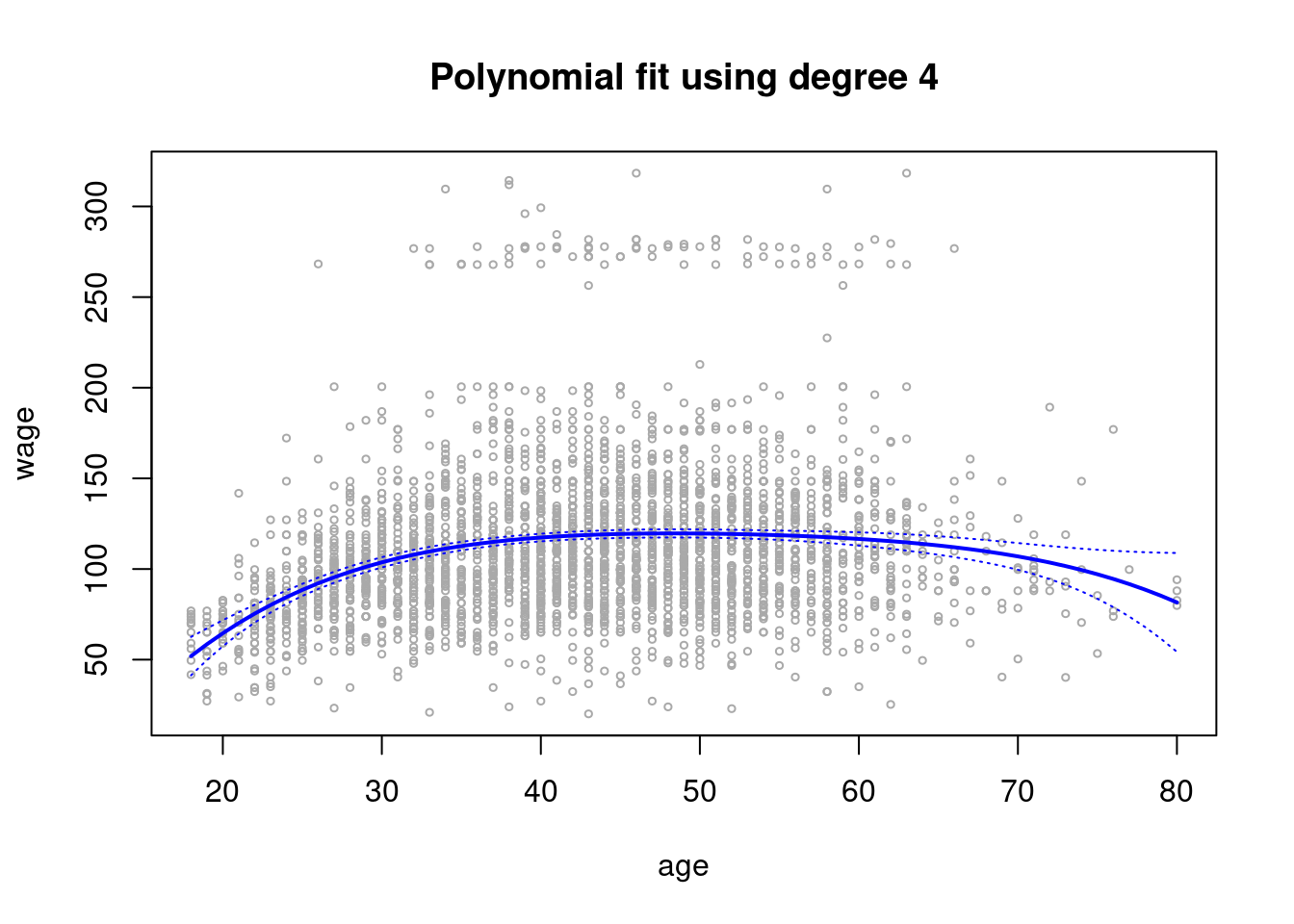
- For step functions
# Cross validation to choose optimal number of cuts.
set.seed(1)
cv.error.20 = rep(NA,19)
for (i in 2:20) {
Wage$age.cut = cut(Wage$age,i)
step.fit=glm(wage~age.cut,data=Wage)
cv.error.20[i-1]=cv.glm(Wage,step.fit,K=10)$delta[1] # [1]: Std [2]: Bias corrected.
}
plot(cv.error.20,type='b',ylab="CV Error")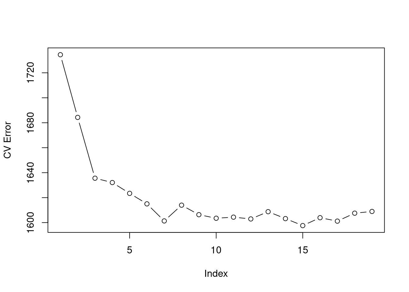
We are advised to use 8 = index + 1 cuts.
step.fit = glm(wage~cut(age,8), data=Wage)
preds2=predict(step.fit,newdata=list(age=age.grid), se=T)
se.bands2=cbind(preds2$fit+2*preds2$se.fit,preds2$fit-2*preds2$se.fit)
plot(age,wage,xlim=agelims,cex=.5,col="darkgrey")
title("Step function using 8 cuts")
lines(age.grid,preds2$fit,lwd=2,col="blue")
matlines(age.grid,se.bands2,lwd =1,col="blue",lty =3)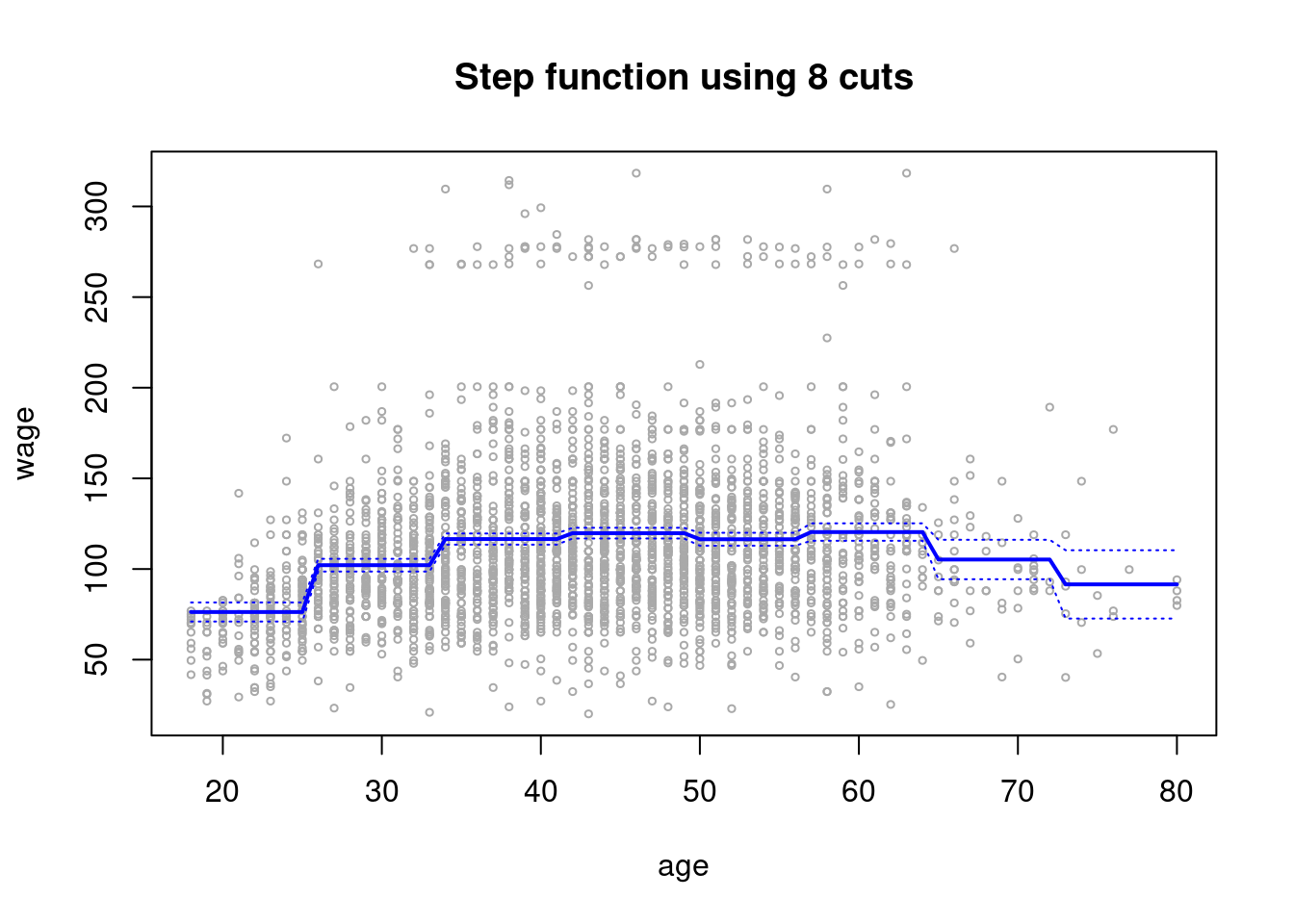
- marital status
Wage |>
  ggplot(aes(x = maritl, y = wage)) +
  geom_boxplot(aes(fill = maritl)) +
  theme_minimal() +
  theme(legend.position = "none")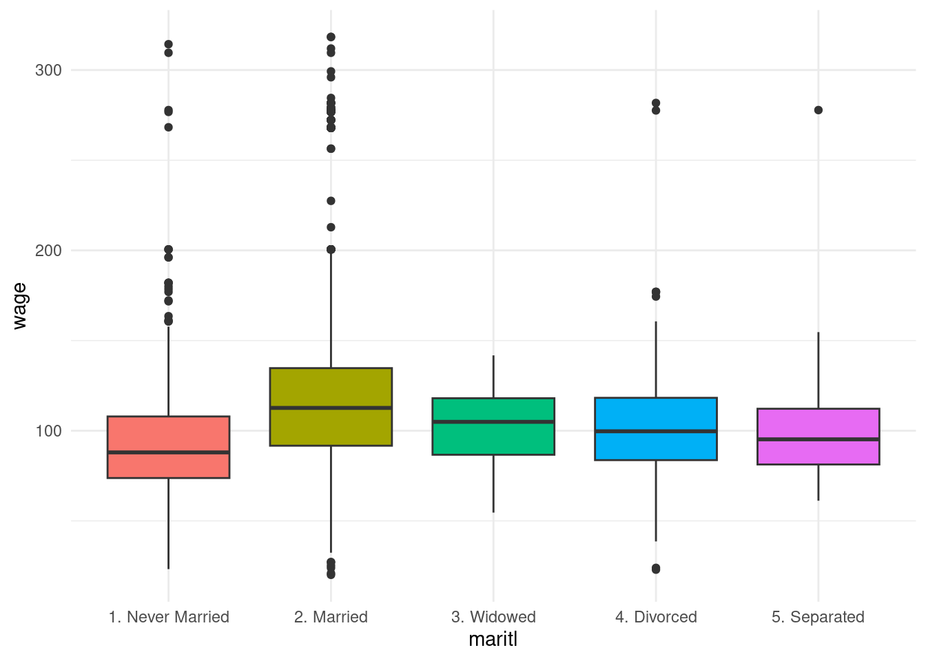
The highest median wage is among married people.
gam.model = gam(wage~maritl, data=Wage)
plot(gam.model, col="blue", se=T)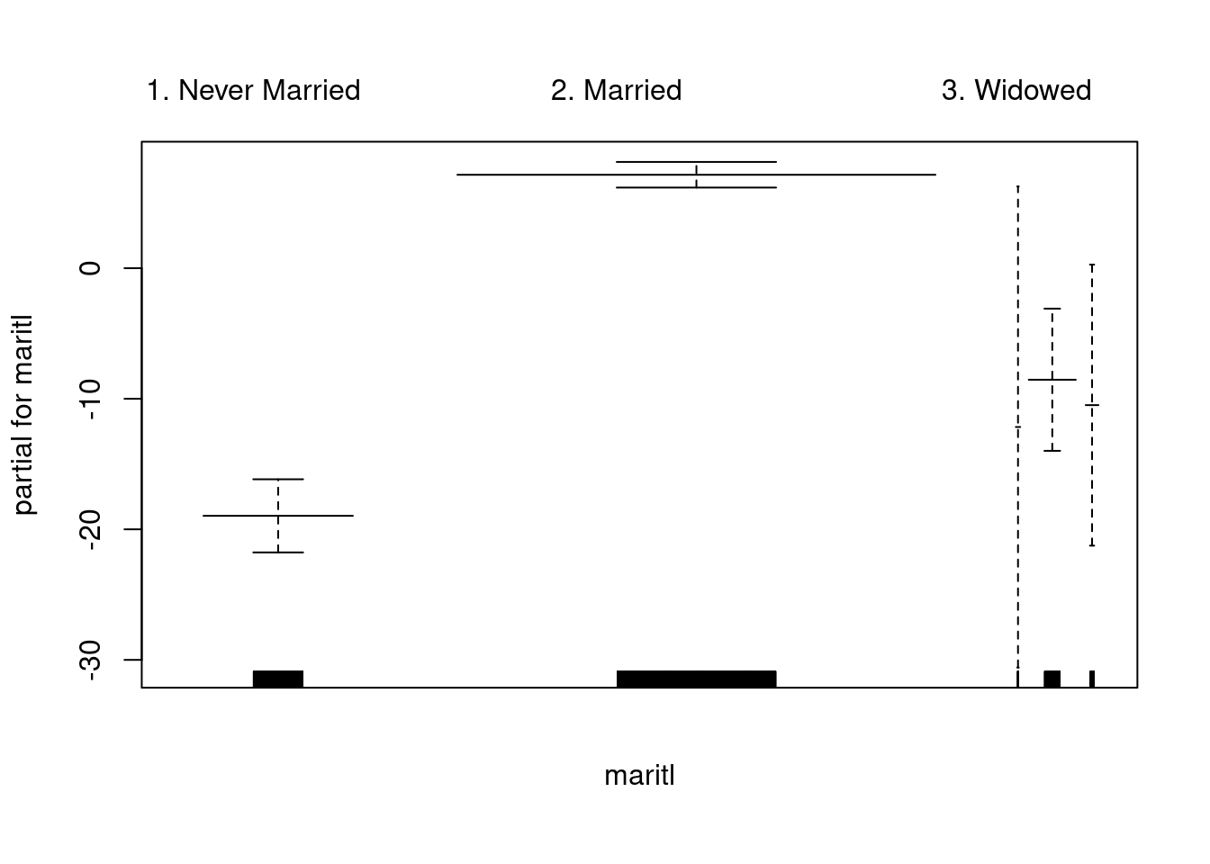
- job class
Wage |>
  ggplot(aes(x = jobclass, y = wage)) +
  geom_boxplot(aes(fill = jobclass)) +
  theme_minimal() +
  theme(legend.position = "none")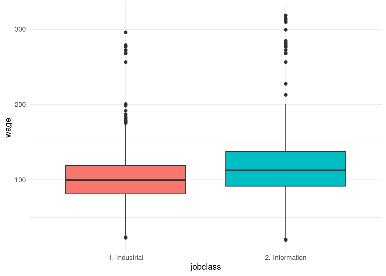
gam_model_2 = gam(wage~jobclass, data=Wage)
plot(gam_model_2, col="blue", se=T)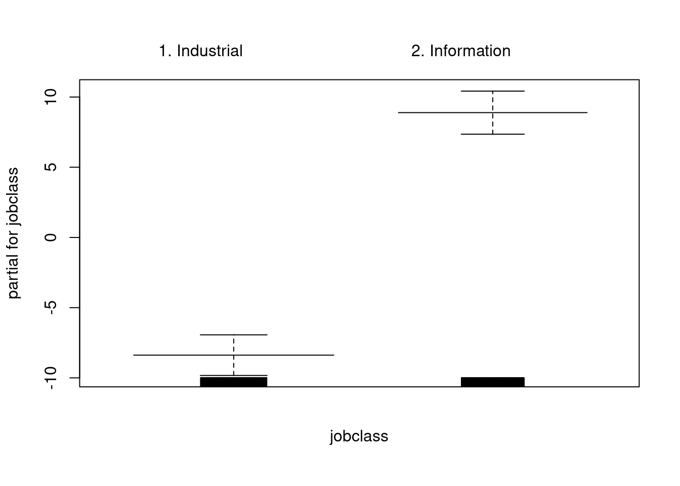
- For the
Autodata set with thempgresponse variable, let us explore nonlinear behavior.
pairs(Auto[1:7])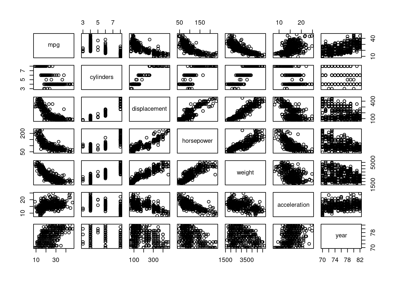
mpgappears to have a non-linear relationship withhorsepower,displacement, andweight
fit.1 = lm(mpg~horsepower ,data=Auto)
fit.2 = lm(mpg~poly(horsepower ,2) ,data=Auto)
fit.3 = lm(mpg~poly(horsepower ,3) ,data=Auto)
fit.4 = lm(mpg~poly(horsepower ,4) ,data=Auto)
fit.5 = lm(mpg~poly(horsepower ,5) ,data=Auto)
fit.6 = lm(mpg~poly(horsepower ,6) ,data=Auto)
anova(fit.1,fit.2,fit.3,fit.4,fit.5,fit.6)
## Analysis of Variance Table
##
## Model 1: mpg ~ horsepower
## Model 2: mpg ~ poly(horsepower, 2)
## Model 3: mpg ~ poly(horsepower, 3)
## Model 4: mpg ~ poly(horsepower, 4)
## Model 5: mpg ~ poly(horsepower, 5)
## Model 6: mpg ~ poly(horsepower, 6)
## Res.Df RSS Df Sum of Sq F Pr(>F)
## 1 390 9385.9
## 2 389 7442.0 1 1943.89 104.6659 < 2.2e-16 ***
## 3 388 7426.4 1 15.59 0.8396 0.360083
## 4 387 7399.5 1 26.91 1.4491 0.229410
## 5 386 7223.4 1 176.15 9.4846 0.002221 **
## 6 385 7150.3 1 73.04 3.9326 0.048068 *
## ---
## Signif. codes: 0 '***' 0.001 '**' 0.01 '*' 0.05 '.' 0.1 ' ' 1- The p-value comparing
fit.1(linear) tofit.2(quadratic) is statistically significant, and the p-value comparingfit.2tofit.3(cubic) is not significant. This indicates that a linear or cubic fit is not sufficient, but a quadratic fit should suffice.
hplim = range(Auto$horsepower)
hp.grid = seq(from=hplim[1],to=hplim[2])
preds1=predict(fit.1,newdata=list(horsepower=hp.grid))
preds2=predict(fit.2,newdata=list(horsepower=hp.grid))
preds5=predict(fit.5,newdata=list(horsepower=hp.grid))
# Plot of linear and polynomial fits.
plot(horsepower,mpg,xlim=hplim,cex.lab=1.5)
lines(hp.grid,preds1,lwd=3,col="blue",lty=2)
lines(hp.grid,preds2,lwd=3,col="red")
lines(hp.grid,preds5,lwd=3,col="green",lty=2)
legend(180,40,legend=c("Linear fit", "Quadratic fit", "Quintic fit"),
col=c("blue", "red", "green"),lty=c(2,1,2), lwd=c(3,3,3),cex=1.5)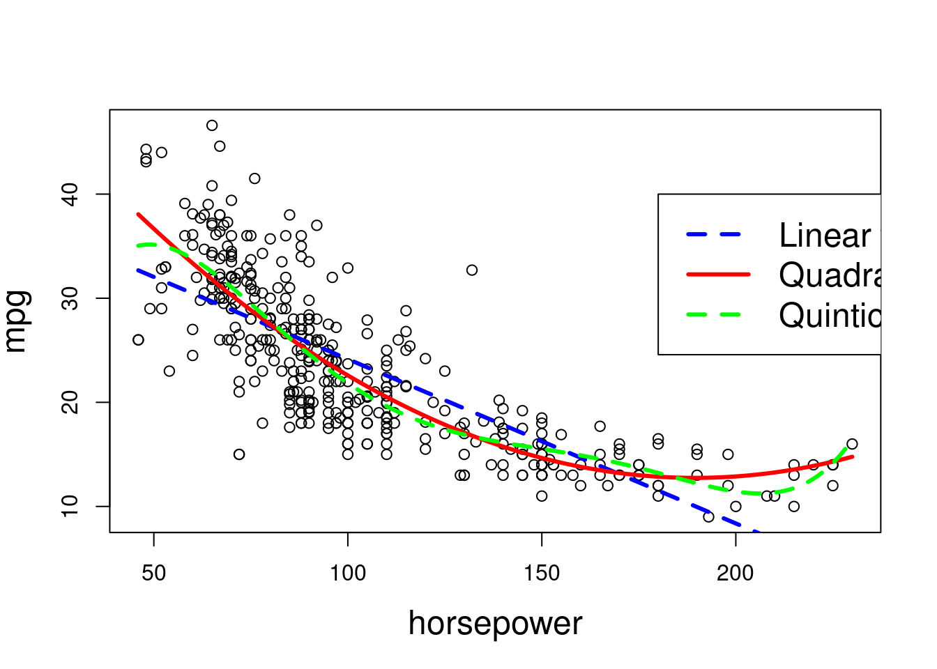
Bostondata
- predictor variable:
nox(nitrogen oxide concentration) - response variable:
dis(distance to employment centers)
- cubic polynomial regression
Boston <- ISLR2::Boston #avoid ambiguity with MASS::Boston
model.1 = glm(nox~poly(dis,3), data=Boston)
plot(Boston$dis,Boston$nox, xlab="Distance", ylab="Nox values")
dis.grid = seq(from=min(Boston$dis),to=max(Boston$dis),0.2)
preds=predict(model.1,newdata=list(dis=dis.grid), se=T)
lines(dis.grid,preds$fit,col="blue",lwd=3)
lines(dis.grid,preds$fit+2*preds$se,col="blue",lwd=3,lty=2)
lines(dis.grid,preds$fit-2*preds$se,col="blue",lwd=3,lty=2)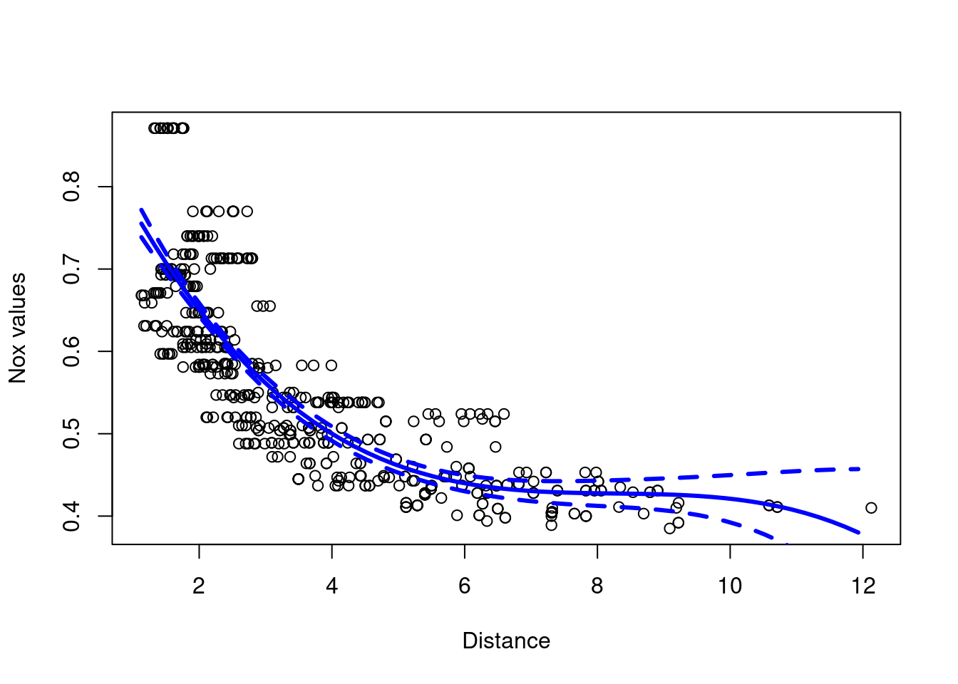
summary(model.1)##
## Call:
## glm(formula = nox ~ poly(dis, 3), data = Boston)
##
## Coefficients:
## Estimate Std. Error t value Pr(>|t|)
## (Intercept) 0.554695 0.002759 201.021 < 2e-16 ***
## poly(dis, 3)1 -2.003096 0.062071 -32.271 < 2e-16 ***
## poly(dis, 3)2 0.856330 0.062071 13.796 < 2e-16 ***
## poly(dis, 3)3 -0.318049 0.062071 -5.124 4.27e-07 ***
## ---
## Signif. codes: 0 '***' 0.001 '**' 0.01 '*' 0.05 '.' 0.1 ' ' 1
##
## (Dispersion parameter for gaussian family taken to be 0.003852802)
##
## Null deviance: 6.7810 on 505 degrees of freedom
## Residual deviance: 1.9341 on 502 degrees of freedom
## AIC: -1370.9
##
## Number of Fisher Scoring iterations: 2- other polynomials
set.seed(2)
boston_df = Boston
# boston_sample = sample.split(boston_df$dis, SplitRatio = 0.80)
boston_sample = sample(c(TRUE, FALSE),
                       replace = TRUE, size = nrow(boston_df),
                       prob = c(0.8, 0.2))
boston_train = subset(boston_df, boston_sample==TRUE)
boston_test = subset(boston_df, boston_sample==FALSE)

rss = rep(0,10)
colours = rainbow(10)
plot(Boston$dis,Boston$nox,xlab="Distance", ylab="Nox values",
main="Polynomial fits from degree 1-10.")
for (i in 1:10){
model = glm(nox~poly(dis,i), data=boston_train)
rss[i] = sum((boston_test$nox - predict(model,newdata=list(dis=boston_test$dis)))^2)
preds=predict(model,newdata=list(dis=dis.grid))
lines(dis.grid,preds,col=colours[i], lwd=2, lty=1)
}
legend(10,0.8,legend=1:10, col= colours[1:10],lty=1,lwd=2)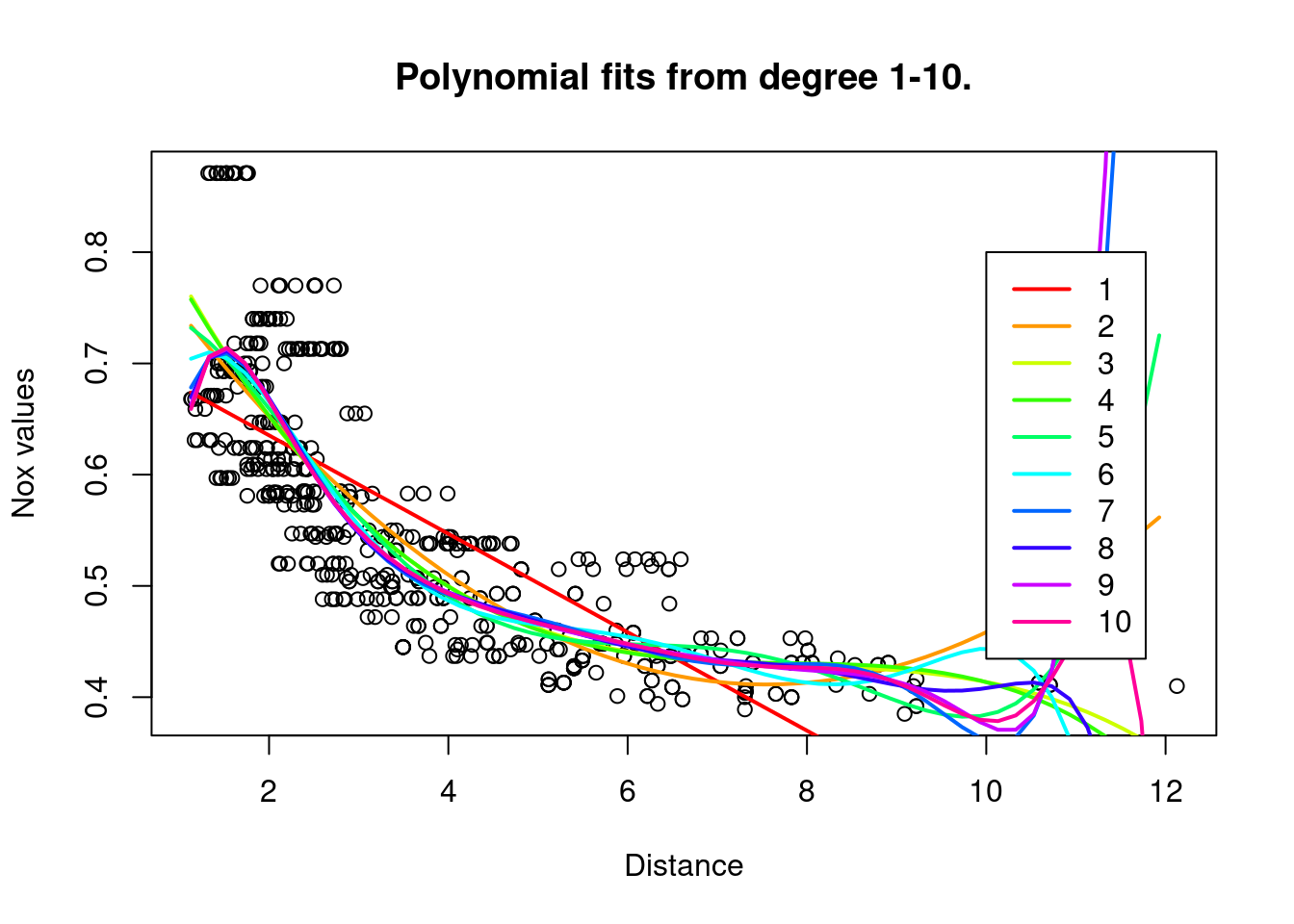
# RSS on the test set.
plot(1:10,rss,xlab="Polynomial degree", ylab="RSS",
main="RSS on test set vs polynomial degree", type='b')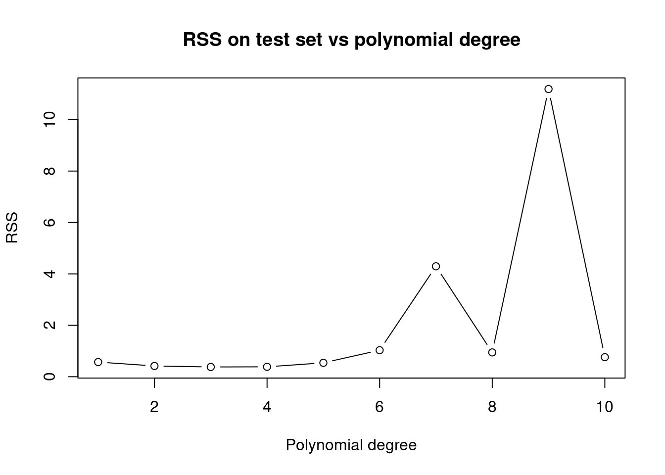
- cross-validation to find polynomial degreee
# Cross validation to choose degree of polynomial.
set.seed(1)
cv.error.10 = rep(0,10)
for (i in 1:10) {
glm.fit=glm(nox~poly(dis,i),data=Boston)
cv.error.10[i]=cv.glm(Boston,glm.fit,K=10)$delta[1]
}
plot(cv.error.10, type="b", xlab="Degree", ylab="CV Error")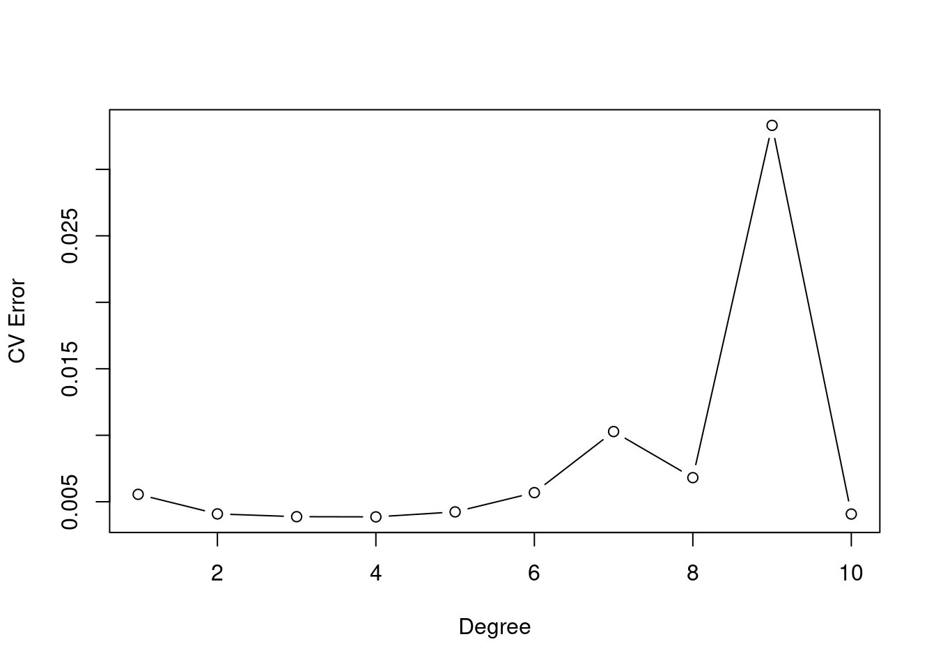
- regression splines
# Regression spline with four degrees of freedom.
spline.fit = lm(nox~bs(dis,df=4), data=Boston)
summary(spline.fit)
##
## Call:
## lm(formula = nox ~ bs(dis, df = 4), data = Boston)
##
## Residuals:
## Min 1Q Median 3Q Max
## -0.124622 -0.039259 -0.008514 0.020850 0.193891
##
## Coefficients:
## Estimate Std. Error t value Pr(>|t|)
## (Intercept) 0.73447 0.01460 50.306 < 2e-16 ***
## bs(dis, df = 4)1 -0.05810 0.02186 -2.658 0.00812 **
## bs(dis, df = 4)2 -0.46356 0.02366 -19.596 < 2e-16 ***
## bs(dis, df = 4)3 -0.19979 0.04311 -4.634 4.58e-06 ***
## bs(dis, df = 4)4 -0.38881 0.04551 -8.544 < 2e-16 ***
## ---
## Signif. codes: 0 '***' 0.001 '**' 0.01 '*' 0.05 '.' 0.1 ' ' 1
##
## Residual standard error: 0.06195 on 501 degrees of freedom
## Multiple R-squared: 0.7164, Adjusted R-squared: 0.7142
## F-statistic: 316.5 on 4 and 501 DF, p-value: < 2.2e-16attr(bs(Boston$dis,df=4),"knots")## [1] 3.20745We have a single knot at the 50th percentile of dis.
plot(Boston$dis,Boston$nox,xlab="Distance", ylab="Nox values")
preds = predict(spline.fit, newdata=list(dis=dis.grid), se=T)
lines(dis.grid, preds$fit,col="red",lwd=3)
lines(dis.grid, preds$fit+2*preds$se,col="blue",lwd=3,lty=2)
lines(dis.grid, preds$fit-2*preds$se,col="blue",lwd=3,lty=2)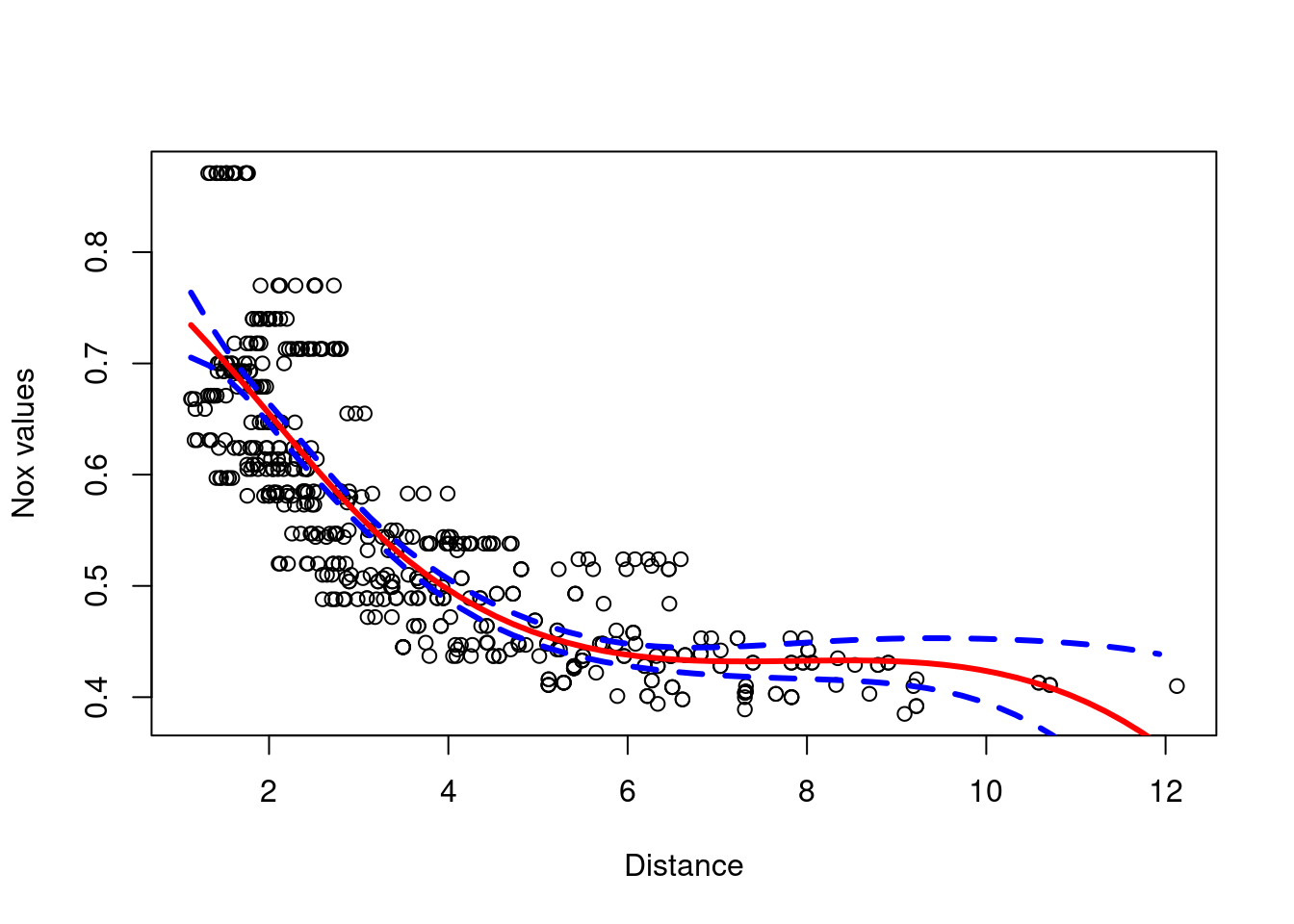
- regression splines over several degrees of freedom
rss = rep(0,18)
colours = rainbow(18)
plot(Boston$dis,Boston$nox,xlab="Distance", ylab="Nox values",
main="Regression splines using degrees from 3-10")
# Degree of freedom starts from 3, anything below is too small.
for (i in 3:20){
spline.model = lm(nox~bs(dis,df=i), data=boston_train)
rss[i-2] = sum((boston_test$nox - predict(spline.model,newdata=list(dis=boston_test$dis)))^2)
preds=predict(spline.model,newdata=list(dis=dis.grid))
lines(dis.grid,preds,col=colours[i-2], lwd=2, lty=1)
}
legend(10,0.8,legend=3:20, col=colours[1:18],lty=1,lwd=2)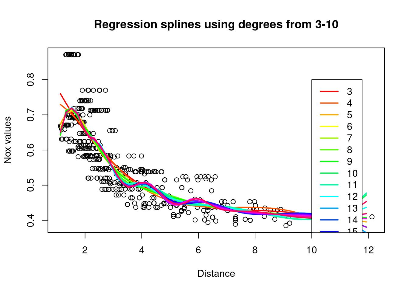
- cross-validation to find the optimal number of degrees of freedom
k=10
set.seed(3)
folds = sample(1:k, nrow(Boston), replace=T)
cv.errors = matrix(NA,k,18, dimnames = list(NULL, paste(3:20))) #CV errors for degrees 3 to 20.
# Create models (total=k) for each degree using the training folds.
# Predict on held out folds and calculate their MSE's(total=k).
# Continue until all j degrees have been used.
# Take the mean of MSE's for each degree.
for(j in 3:20){
for(i in 1:k){
spline.model=lm(nox~bs(dis,df=j), data=Boston[folds!=i,])
pred=predict(spline.model,Boston[folds==i,],id=i)
cv.errors[i,j-2]=mean((Boston$nox[folds==i] - pred)^2)
}
}
mean.cv.errors = apply(cv.errors,2,mean)
mean.cv.errors[which.min(mean.cv.errors)]
## 8
## 0.003693139Our calculations point toward a degree-8 polynomial.
- For the
Collegedata set
- response variable:
Outstate - predictor variables: [all other variables]
- forward stepwise selection
set.seed(4)
college_df = College
# college_sample = sample.split(college_df$Outstate, SplitRatio = 0.80)
college_sample = sample(c(TRUE, FALSE),
                        replace = TRUE, size = nrow(college_df),
                        prob = c(0.8, 0.2))
college_train = subset(college_df, college_sample==TRUE)
college_test = subset(college_df, college_sample==FALSE)

# Forward stepwise on the training set using all variables.
fit.fwd = regsubsets(Outstate~., data=college_train, nvmax=17, method="forward")
fit.summary = summary(fit.fwd)
# Some Statistical metrics.
which.min(fit.summary$bic) #Estimate of the test error, lower is better.
## [1] 10par(mfrow=c(2,2))
plot(1:17, fit.summary$cp,xlab="Variables",ylab="Cp",main="Cp", type='b')
plot(1:17, fit.summary$bic,xlab="Variables",ylab="BIC",main="BIC", type='b')
plot(1:17, fit.summary$adjr2,xlab="Variables",ylab="Adjusted R2",main="Adjusted R2", type='b')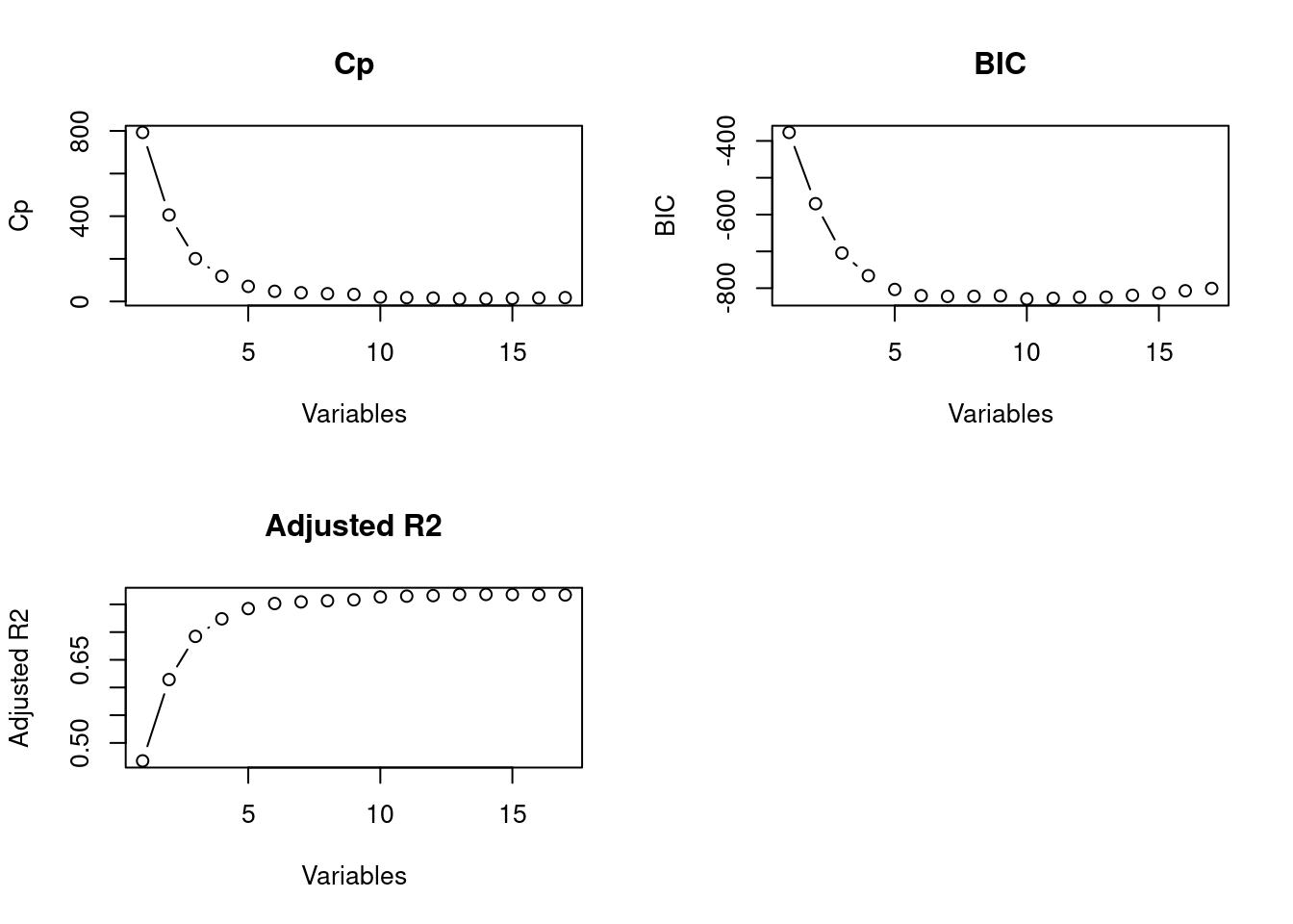
coef(fit.fwd,6)## (Intercept) PrivateYes Room.Board PhD perc.alumni
## -3601.7165495 2804.7790744 0.9479096 39.9003543 41.5638460
## Expend Grad.Rate
## 0.2275343 28.4405943- GAM (generalized additive model)
gam.m1 = gam(Outstate~Private+
               s(Room.Board,4)+
               s(PhD,4)+
               s(perc.alumni,2)+
               s(Expend,4)+
               s(Grad.Rate,5), data=college_train)
par(mfrow=c(2,3))
plot(gam.m1, col="blue", se=T)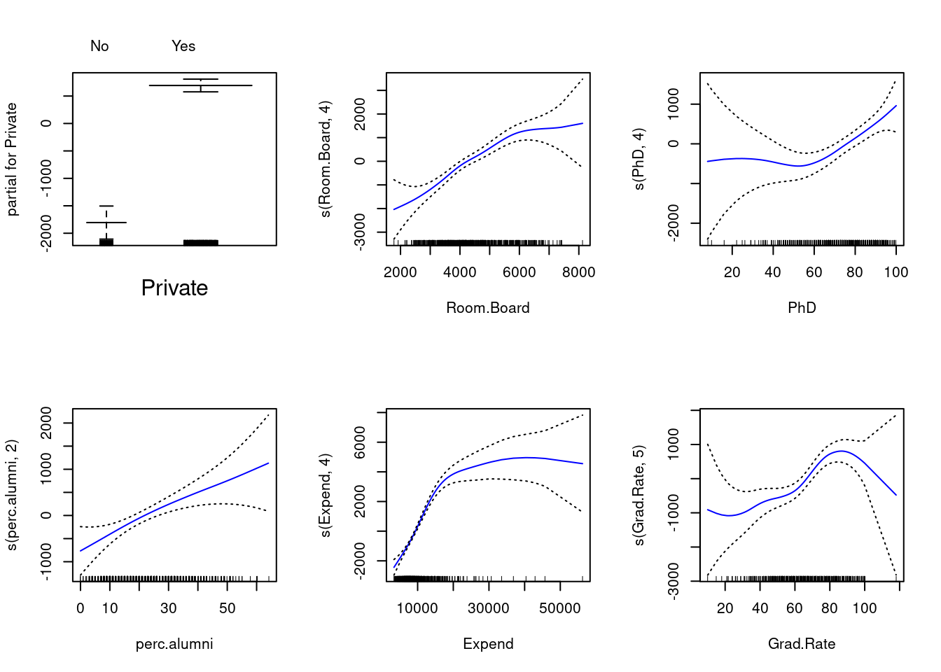
- model statistics
gam.m2 = gam(Outstate~Private+s(Room.Board,4)+s(PhD,4)+s(perc.alumni,2)
+s(Expend,4), data=college_train) # No Grad.Rate
gam.m3 = gam(Outstate~Private+s(Room.Board,4)+s(PhD,4)+s(perc.alumni,2)
+s(Expend,4)+Grad.Rate, data=college_train) # Linear Grad rate
gam.m4 = gam(Outstate~Private+s(Room.Board,4)+s(PhD,4)+s(perc.alumni,2)
+s(Expend,4)+s(Grad.Rate,4), data=college_train) # Spline with 4 degrees
anova(gam.m2,gam.m3,gam.m4,gam.m1, test="F")
## Analysis of Deviance Table
##
## Model 1: Outstate ~ Private + s(Room.Board, 4) + s(PhD, 4) + s(perc.alumni,
## 2) + s(Expend, 4)
## Model 2: Outstate ~ Private + s(Room.Board, 4) + s(PhD, 4) + s(perc.alumni,
## 2) + s(Expend, 4) + Grad.Rate
## Model 3: Outstate ~ Private + s(Room.Board, 4) + s(PhD, 4) + s(perc.alumni,
## 2) + s(Expend, 4) + s(Grad.Rate, 4)
## Model 4: Outstate ~ Private + s(Room.Board, 4) + s(PhD, 4) + s(perc.alumni,
## 2) + s(Expend, 4) + s(Grad.Rate, 5)
## Resid. Df Resid. Dev Df Deviance F Pr(>F)
## 1 601 2166323188
## 2 600 2066713778 1.00000 99609410 29.2509 9.217e-08 ***
## 3 597 2035360253 3.00016 31353525 3.0689 0.02744 *
## 4 596 2029589922 0.99959 5770331 1.6952 0.19342
## ---
## Signif. codes: 0 '***' 0.001 '**' 0.01 '*' 0.05 '.' 0.1 ' ' 1- Here we explore backfitting i the context of multiple linear regression. Suppose that we build an approach below and converge on coefficients.
- Generate a response \(Y\) from two predictors \(X_{1}\) and \(X_{2}\) with \(n = 100\)
set.seed(5)
# Generated dataset
X1 = rnorm(100, sd=2)
X2 = rnorm(100, sd=sqrt(2))
eps = rnorm(100, sd = 1)
b0 = 5; b1=2.5 ; b2=11.5
Y = b0 +b1*X1 + b2*X2 + eps- Initialize \(\hat{\beta}_{1}\) with some value, then with \(\hat{\beta}_{1}\) fixed, fit the model
\[Y - \hat{\beta}_{1}X_{1} = \beta_{0} + \beta_{2}X_{2} + \epsilon\]
beta1 = 0.1
a=Y-beta1*X1
beta2=lm(a~X2)$coef[2]
beta2
## X2
## 11.90966- Keeping \(\hat{\beta}_{2}\) fixed, fit the model
\[Y - \hat{\beta}_{2}X_{2} = \beta_{0} + \beta_{1}X_{1} + \epsilon\]
a=Y-beta2*X2
beta1 = lm(a~X1)$coef[2]
beta1
## X1
## 2.49134- loop
beta.df = data.frame("beta0"=rep(0,1000),"beta1"=rep(0,1000),"beta2"=rep(0,1000))
beta1 = 0.1
for (i in 1:1000){
a=Y-beta1*X1
model = lm(a~X2)
beta2 = model$coef[2]
beta.df$beta2[i]= beta2
a=Y-beta2*X2
model = lm(a~X1)
beta1 = model$coef[2]
beta.df$beta1[i]=beta1
beta.df$beta0[i]=model$coef[1]
}
# Beta values after 5 iterations.
print(c(beta.df$beta0[5], beta.df$beta1[5], beta.df$beta2[5]))
## [1] 4.996049 2.526440 11.536752- compare to multiple linear regression
lm.fit = lm(Y~X1+X2)
coef(lm.fit)
## (Intercept) X1 X2
## 4.996049 2.526440 11.536752- Here we approximate multiple linear regression by repeatedly performing simple linear regression in a backfitting procedure.
set.seed(6)
n = 1000 # Number of examples
p = 100 # Number of predictors
# Generated dataset
X = matrix(rnorm(n*p),n,p)
beta0 = 8
betas = rnorm(100, sd = 2)
eps = rnorm(100, sd = 1)

Y = beta0 + X%*%betas + eps

bhats = matrix(0,nrow=25,ncol=100)
intercepts = matrix(0,25,1)
# For loop to create models(M) that excludes the predictors that are 'fixed',
# and uses lm() to estimate the coefficent of the unfixed predictor.
# Estimates are stored such that the values can be used for the next set of calculations.
for (i in 1:25){
for(j in 1:100){
# Matrix multiplication of the fixed predictors and their respective coefficient estimates.
M = Y - (X[,-j] %*% bhats[i,-j])
# Linear regression with results stored in all rows from row(i):row(end).
bhats[i:25,j] = lm(M~X[,j])$coef[2]
intercepts[i] = lm(M~X[,j])$coef[1]
}
}- via base-R multiple linear regression
lm.fit = lm(Y~X)
# Intercept and selected coefficient values.
print(c(coef(lm.fit)[1], coef(lm.fit)[2], coef(lm.fit)[10], coef(lm.fit)[20]))
## (Intercept) X1 X9 X19
## 7.9629583 -2.6797748 -0.7035457 3.4133121- via the improvised algorithm
# Intercept, and selected coefficient values after iterating 25 times.
print(c(intercepts[25], bhats[25,1], bhats[25,9], bhats[25,19]))
## [1] 7.9629583 -2.6797748 -0.7035457 3.4133121