9.13 Lab: Support Vector Classifier
library("tidymodels")
library("kernlab") # We'll use the plot method from this.set.seed(1)
sim_data <- matrix(
rnorm (20 * 2),
ncol = 2,
dimnames = list(NULL, c("x1", "x2"))
) %>%
as_tibble() %>%
mutate(
y = factor(c(rep(-1, 10), rep(1, 10)))
) %>%
mutate(
x1 = ifelse(y == 1, x1 + 1, x1),
x2 = ifelse(y == 1, x2 + 1, x2)
)
sim_data %>%
ggplot() +
aes(x1, x2, color = y) +
geom_point() +
labs(title = "Trying to make a hyperplane classifier",
subtitle = "simulated data",
caption = "R4DS book club") +
theme_minimal()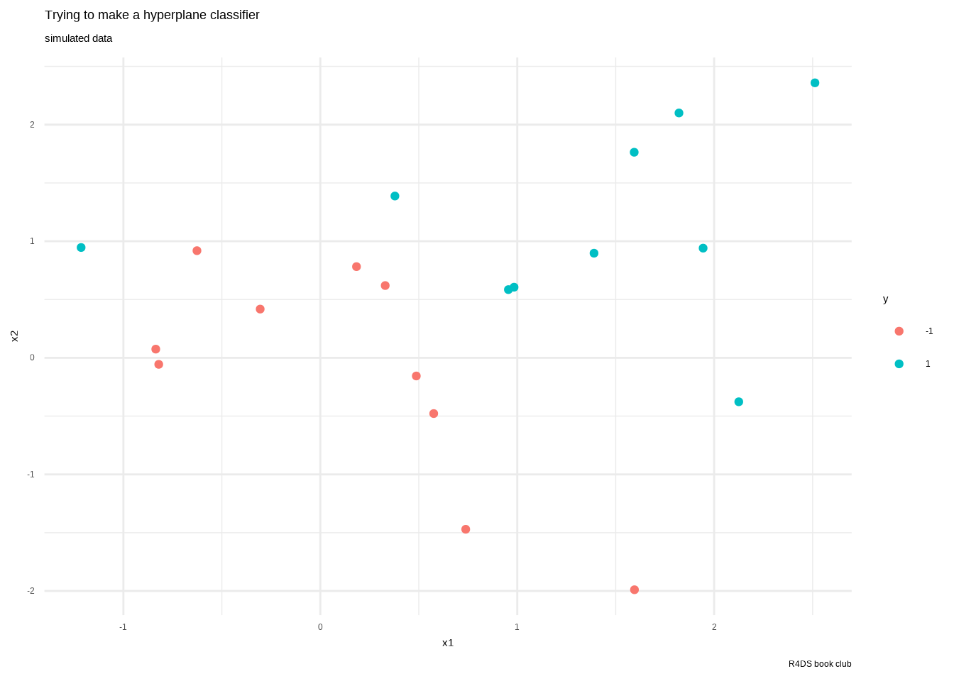
# generated this using their process then saved it to use here.
test_data <- readRDS("data/09-testdat.rds") %>%
  rename(x1 = x.1, x2 = x.2)

test_data %>%
  ggplot() +
  aes(x1, x2, color = y) +
  geom_point() +
  labs(title = "Trying to make a hyperplane classifier",
       subtitle = "simulated data",
       caption = "R4DS book club") +
  theme_minimal()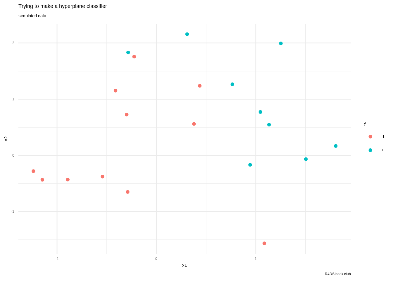
We create a spec for a model, which we’ll update throughout this lab with different costs.
svm_linear_spec <- svm_poly(degree = 1) %>%
  set_mode("classification") %>%
  set_engine("kernlab", scaled = FALSE)
Then we do a couple fits with manual cost.
svm_linear_fit_10 <- svm_linear_spec %>%
  set_args(cost = 10) %>%
  fit(y ~ ., data = sim_data)
svm_linear_fit_10
## parsnip model object
##
## Support Vector Machine object of class "ksvm"
##
## SV type: C-svc (classification)
## parameter : cost C = 10
##
## Polynomial kernel function.
## Hyperparameters : degree = 1 scale = 1 offset = 1
##
## Number of Support Vectors : 7
##
## Objective Function Value : -52.4483
## Training error : 0.15
## Probability model included.svm_linear_fit_10 %>%
extract_fit_engine() %>%
plot()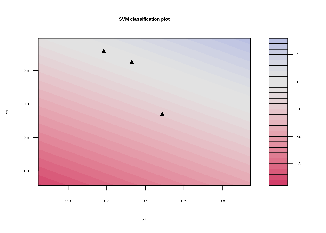
svm_linear_fit_01 <- svm_linear_spec %>%
  set_args(cost = 0.1) %>%
  fit(y ~ ., data = sim_data)
svm_linear_fit_01
## parsnip model object
##
## Support Vector Machine object of class "ksvm"
##
## SV type: C-svc (classification)
## parameter : cost C = 0.1
##
## Polynomial kernel function.
## Hyperparameters : degree = 1 scale = 1 offset = 1
##
## Number of Support Vectors : 16
##
## Objective Function Value : -1.189
## Training error : 0.05
## Probability model included.svm_linear_fit_01 %>%
extract_fit_engine() %>%
plot()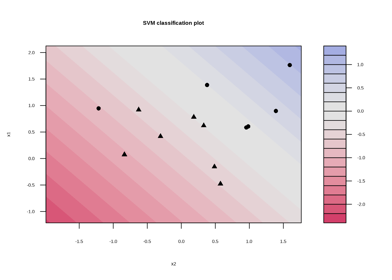
svm_linear_fit_001 <- svm_linear_spec %>%
  set_args(cost = 0.01) %>%
  fit(y ~ ., data = sim_data)
svm_linear_fit_001
## parsnip model object
##
## Support Vector Machine object of class "ksvm"
##
## SV type: C-svc (classification)
## parameter : cost C = 0.01
##
## Polynomial kernel function.
## Hyperparameters : degree = 1 scale = 1 offset = 1
##
## Number of Support Vectors : 20
##
## Objective Function Value : -0.1859
## Training error : 0.25
## Probability model included.svm_linear_fit_001 %>%
extract_fit_engine() %>%
plot()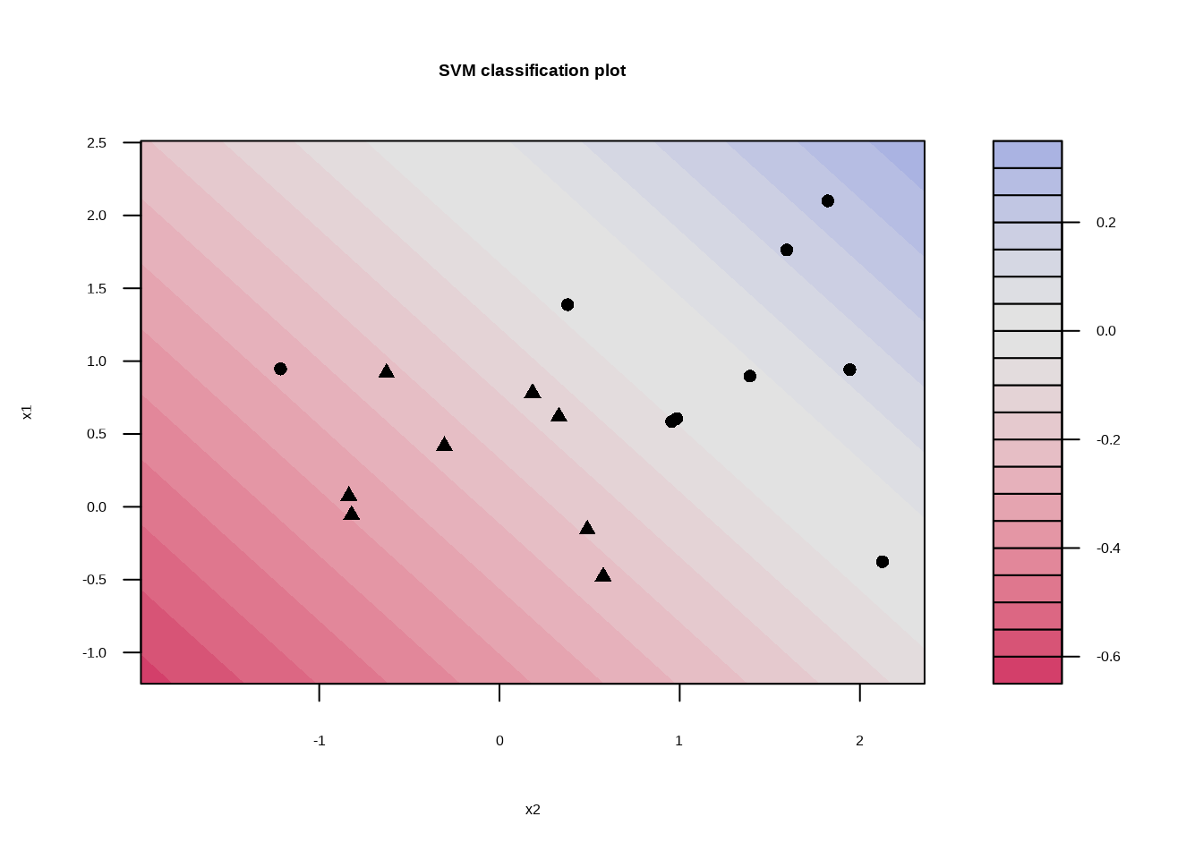
9.13.1 Tuning
Let’s find the best cost.
svm_linear_wf <- workflow() %>%
  add_model(
    svm_linear_spec %>% set_args(cost = tune())
  ) %>%
  add_formula(y ~ .)

set.seed(1234)
sim_data_fold <- vfold_cv(sim_data, strata = y)

param_grid <- grid_regular(cost(), levels = 10)

# Our grid isn't identical to the book, but it's close enough.
param_grid
## # A tibble: 10 × 1
## cost
## <dbl>
## 1 0.000977
## 2 0.00310
## 3 0.00984
## 4 0.0312
## 5 0.0992
## 6 0.315
## 7 1
## 8 3.17
## 9 10.1
## 10 32tune_res <- tune_grid(
svm_linear_wf,
resamples = sim_data_fold,
grid = param_grid
)
# We ran this locally and then saved it so everyone doesn't need to wait for
# this to process each time they build the book.
# saveRDS(tune_res, "data/09-tune_res.rds")autoplot(tune_res)Tune can pull out the best result for us.
best_cost <- select_best(tune_res, metric = "accuracy")

svm_linear_final <- finalize_workflow(svm_linear_wf, best_cost)

svm_linear_fit <- svm_linear_final %>% fit(sim_data)

svm_linear_fit %>%
  augment(new_data = test_data) %>%
  conf_mat(truth = y, estimate = .pred_class)
## Truth
## Prediction -1 1
## -1 9 1
## 1 2 8\[\text{accuracy} = \frac{9 + 8}{9 + 1 + 2 + 8} = 0.85\]
svm_linear_fit_001 %>%
  augment(new_data = test_data) %>%
  conf_mat(truth = y, estimate = .pred_class)
## Truth
## Prediction -1 1
## -1 11 6
## 1 0 3\[\text{accuracy} = \frac{11 + 3}{11 + 6 + 0 + 3} = 0.70\]
9.13.2 Linearly separable data
sim_data_sep <- sim_data %>%
  mutate(
    x1 = ifelse(y == 1, x1 + 0.5, x1),
    x2 = ifelse(y == 1, x2 + 0.5, x2)
  )

sim_data_sep %>%
  ggplot() +
  aes(x1, x2, color = y) +
  geom_point()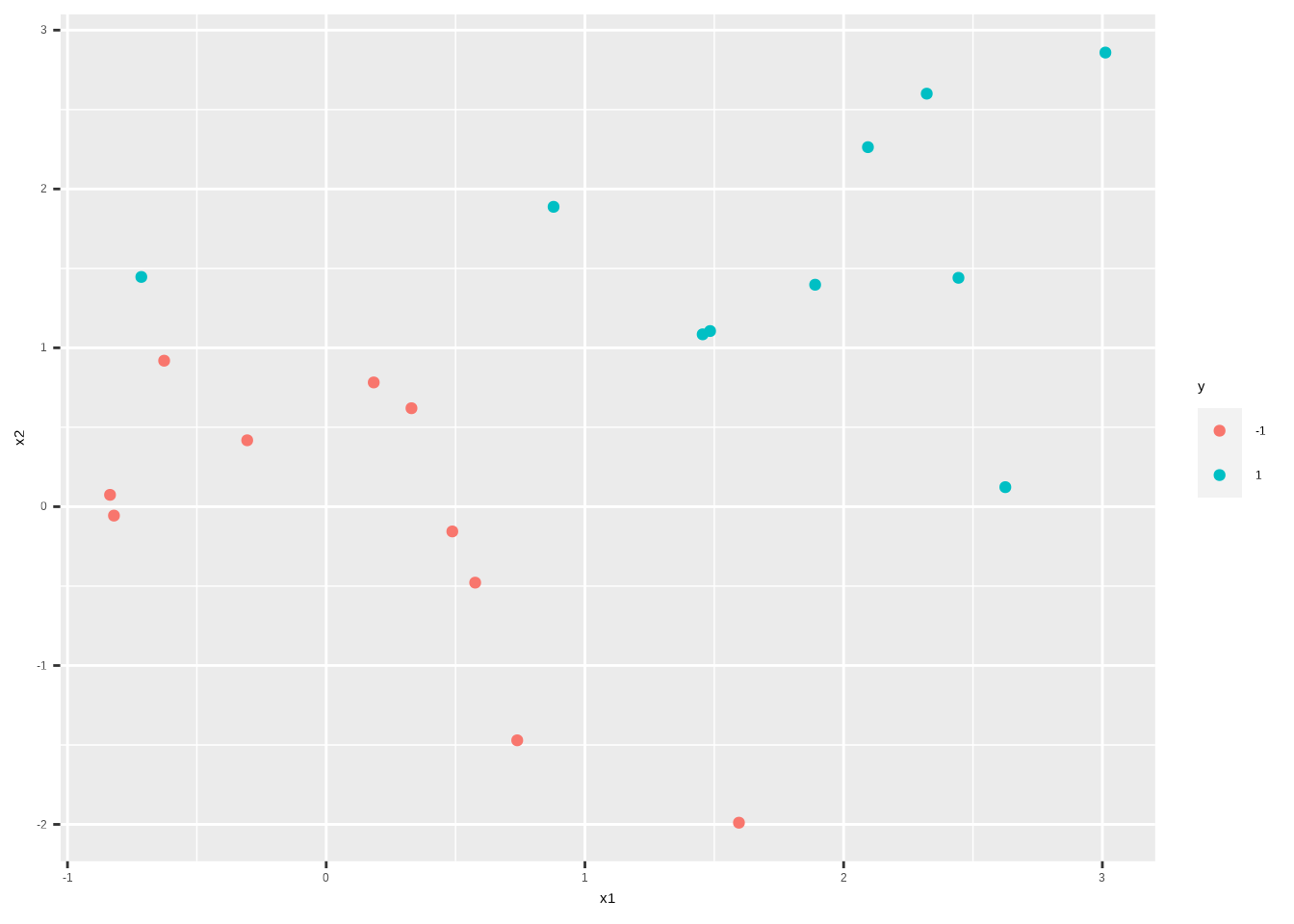
svm_fit_sep_1e5 <- svm_linear_spec %>%
  set_args(cost = 1e5) %>%
  fit(y ~ ., data = sim_data_sep)

svm_fit_sep_1e5
## parsnip model object
##
## Support Vector Machine object of class "ksvm"
##
## SV type: C-svc (classification)
## parameter : cost C = 1e+05
##
## Polynomial kernel function.
## Hyperparameters : degree = 1 scale = 1 offset = 1
##
## Number of Support Vectors : 3
##
## Objective Function Value : -24.3753
## Training error : 0
## Probability model included.svm_fit_sep_1e5 %>%
extract_fit_engine() %>%
plot()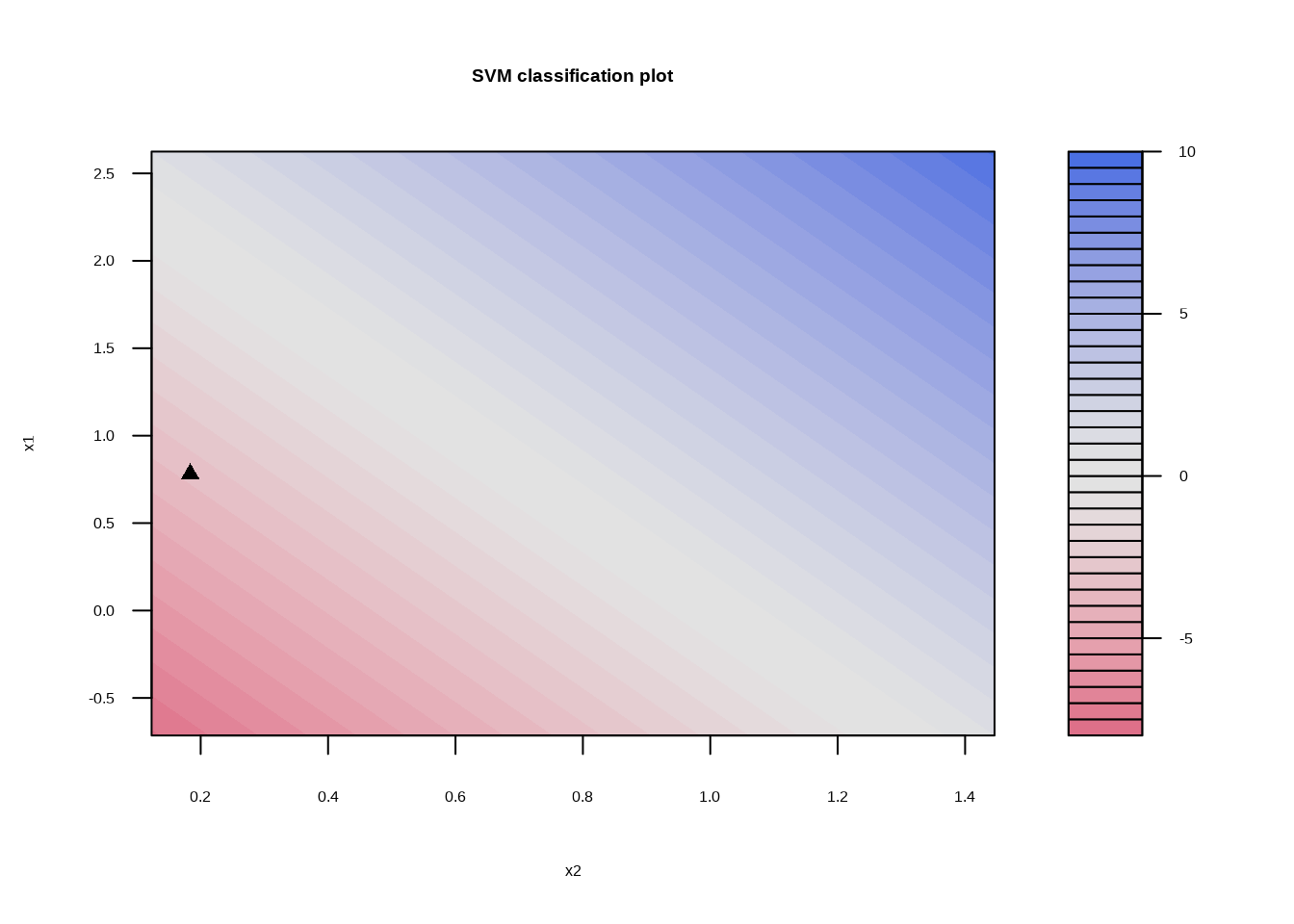
svm_fit_sep_1 <- svm_linear_spec %>%
  set_args(cost = 1) %>%
  fit(y ~ ., data = sim_data_sep)

svm_fit_sep_1
## parsnip model object
##
## Support Vector Machine object of class "ksvm"
##
## SV type: C-svc (classification)
## parameter : cost C = 1
##
## Polynomial kernel function.
## Hyperparameters : degree = 1 scale = 1 offset = 1
##
## Number of Support Vectors : 7
##
## Objective Function Value : -3.5451
## Training error : 0.05
## Probability model included.svm_fit_sep_1 %>%
extract_fit_engine() %>%
plot()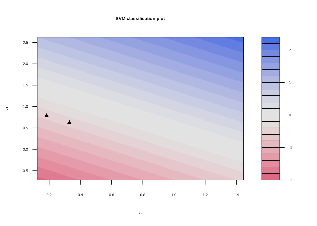
test_data_sep <- test_data %>%
  mutate(
    x1 = ifelse(y == 1, x1 + 0.5, x1),
    x2 = ifelse(y == 1, x2 + 0.5, x2)
  )

svm_fit_sep_1e5 %>%
  augment(new_data = test_data_sep) %>%
  conf_mat(truth = y, estimate = .pred_class)
## Truth
## Prediction -1 1
## -1 9 1
## 1 2 8\[\text{accuracy} = \frac{9 + 8}{8 + 1 + 2 + 8} = 0.85\]
svm_fit_sep_1 %>%
  augment(new_data = test_data_sep) %>%
  conf_mat(truth = y, estimate = .pred_class)
## Truth
## Prediction -1 1
## -1 9 0
## 1 2 9\[\text{accuracy} = \frac{9 + 9}{9 + 0 + 2 + 9} = 0.90\]