4.3 Logistic Regression
4.3.1 The Logistic Model
- Logistic regression: models the probability that Y belongs to a particular category (X)
- X is binary (0/1)
\[p(X) = β_0 + β_1X \space \Longrightarrow {Linear \space regression}\] \[p (X) = \frac{e^{\beta_{0} + \beta_{1}X}}{1 + e^{\beta_{0} + \beta_{1}X}} \space \Longrightarrow {Logistic \space function}\] \[odds = \frac{p (X)}{1 - p (X)} = e^{\beta_{0} + \beta_{1}X} \Longrightarrow {odds \space value [0, ∞]}\]
By logging the whole equation, we get
\[\log \biggl(\frac{p(X)}{1- p(X)}\bigg) = \beta_{0} + \beta_{1}X \Longrightarrow {log \space odds/logit}\]
4.3.2 Estimating the Regression Coefficient
To estimate the regression coefficient, we use maximum likelihood (ME).
Likelihood Function
\[ℓ (\beta_{0}, \beta_{1}) = \prod_{i: y_{i}= 1} p (x_i) \prod_{i': y_{i'}= 0} (1- p (x_{i'})) \Longrightarrow {Likelihood \space function}\]
- The aim is to find beta values such that \[ℓ\] is maximum.
- The Least square method is the special case of maximum likelihood function.
4.3.3 Multiple Logistic Regression
\[\log \biggl(\frac{p(X)}{1- p(X)}\bigg) = \beta_{0} + \beta_{1}X_1 + ... + \beta_{p}X_p \\ \Downarrow \\ p(X) = \frac{e^{\beta_{0} + \beta_{1}X_1 + ... + \beta_{p}X_p}}{1 + \beta_{0} + \beta_{1}X_1 + ... + \beta_{p}X_p}\]
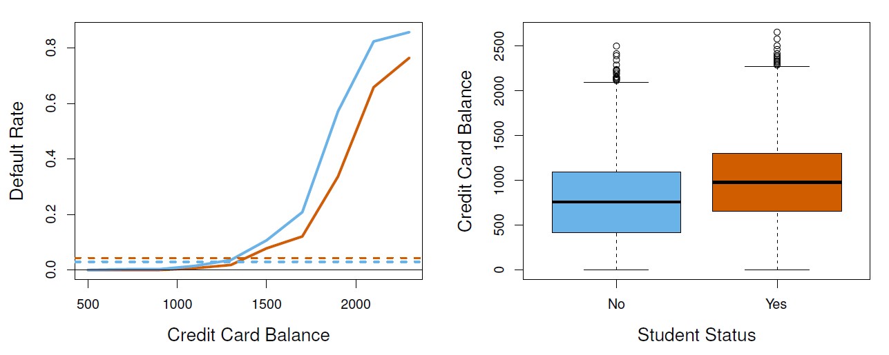
Figure 4.3: Confounding in the Default data. Left: Default rates are shown for students (orange) and non-students (blue). The solid lines display default rate as a function of balance, while the horizontal broken lines display the overall default rates. Right: Boxplots of balance for students (orange) and non-students (blue) are shown.
4.3.4 Multinomial Logistic Regression
This is used in the setting where K > 2 classes. In multinomial, we select a single class to serve as the baseline.
However, the interpretation of the coefficients in a multinomial logistic regression model must be done with care, since it is tied to the choice of baseline.
Alternatively, you can use `Softmax coding, where we treat all K classes symmetrically, and assume that for k = 1, . . . ,K, rather than selecting a baseline. This means, we estimate coefficients for all K classes, rather than estimating coefficients for K − 1 classes.