4.19 Exercises
4.19.1 Conceptual
- Claim: The logistic function representation for logistic regression
\[p (X) = \frac{e^{\beta_{0} + \beta_{1}X}}{1 + e^{\beta_{0} + \beta_{1}X}} \space \Longrightarrow {Logistic \space function}\]
is equivalent to the logit function representation for logistic regression.
\[\log \biggl(\frac{p(X)}{1- p(X)}\bigg) = \beta_{0} + \beta_{1}X \Longrightarrow {log \space odds/logit}\]
Proof:
\[\begin{array}{rcl} p(X) & = & \frac{e^{\beta_{0} + \beta_{1}X}}{1 + e^{\beta_{0} + \beta_{1}X}} \\ p(X)[1 + e^{\beta_{0} + \beta_{1}X}] & = & e^{\beta_{0} + \beta_{1}X} \\ p(X) + p(X)e^{\beta_{0} + \beta_{1}X} & = & e^{\beta_{0} + \beta_{1}X} \\ p(X) & = & e^{\beta_{0} + \beta_{1}X} - p(X)e^{\beta_{0} + \beta_{1}X} \\ p(X) & = & e^{\beta_{0} + \beta_{1}X}[1 - p(X)] \\ \frac{p(X)}{1 - p(X)} & = & e^{\beta_{0} + \beta_{1}X} \\ \log \biggl(\frac{p(X)}{1- p(X)}\bigg) & = & \beta_{0} + \beta_{1}X \\ \end{array}\]
- Under the assumption that the observations in the \(k^{th}\) class are drawn from a Gaussian \(N(\mu_{k}, \sigma^{2})\) distribution,
\[p_k(x) = \frac{π_k \frac{1}{\sqrt{2πσ}}exp(- \frac{1}{2σ^2}(x- \mu_k)^2)}{\sum^k_{l=1} π_l \frac{1}{\sqrt{2πσ}}exp(- \frac{1}{2σ^2}(x- \mu_l)^2)}\]
is largest when \(x = \mu_{k}\) (i.e. observation classified when \(x\) is close to \(\mu_{k}\)). We can proceed toward the discriminant function \(\delta_{k}(x) = \ln C^{-1}p_{k}(x)\) using \(C\) as a scaling factor of proportionality
\[\begin{array}{rcl} p_k(x) & = & \frac{π_k \frac{1}{\sqrt{2πσ}}exp(- \frac{1}{2σ^2}(x- \mu_k)^2)}{\sum^k_{l=1} π_l \frac{1}{\sqrt{2πσ}}exp(- \frac{1}{2σ^2}(x- \mu_l)^2)} \\ p_k(x) & \propto & π_k \frac{1}{\sqrt{2πσ}}exp(- \frac{1}{2σ^2}(x- \mu_k)^2) \\ p_k(x) & \propto & π_k \frac{1}{\sqrt{2πσ}}exp(- \frac{1}{2σ^2}(x^{2}- 2\mu_{k}x + \mu_{k}^{2})) \\ p_k(x) & = & Cπ_k exp(- \frac{1}{2σ^2}(-2\mu_{k}x + \mu_{k}^{2})) \\ C^{-1}p_k(x) & = & π_k exp(- \frac{1}{2σ^2}(-2\mu_{k}x + \mu_{k}^{2})) \\ \ln C^{-1}p_{k}(x) & = & \ln \pi_{k} + \frac{\mu_{k}x}{\sigma^{2}} - \frac{\mu_{k}^{2}}{2\sigma^{2}} \\ \delta_{k}(x) & = & \frac{\mu_{k}x}{\sigma^{2}} - \frac{\mu_{k}^{2}}{2\sigma^{2}} + \ln \pi_{k} \end{array}\]
where the observation is also classified into the \(k^{th}\) class when \(x\) is close to \(\mu_{k}\).
- For QDA, whose observations \(X_{k} \sim N(\mu_{k}, \sigma_{k}^{2})\), consider the case with one feature (i.e. \(p = 1\)). Prove that the Bayes Classifier is quadratic (i.e. not linear).
In a similar proof as the previous exercise, but without the assumption of the same variance, so each class has its own variance \(\sigma_{k}\),
\[p_k(x) = \frac{π_k \frac{1}{\sqrt{2πσ_{k}}}exp(- \frac{1}{2σ_{k}^2}(x- \mu_k)^2)}{\sum^k_{l=1} π_l \frac{1}{\sqrt{2πσ_{l}}}exp(- \frac{1}{2σ_{l}^2}(x- \mu_l)^2)}\] and we would arrive at the discriminant function
\[\begin{array}{rcl} C^{-1}p_k(x) & = & \frac{\pi_k}{\sigma_{k}} exp(- \frac{1}{2σ_{k}^2}(x^{2}-2\mu_{k}x + \mu_{k}^{2})) \\ \ln C^{-1}p_{k}(x) & = & \ln\frac{π_k}{\sigma_{k}} - \frac{x^{2}}{2\sigma_{k}^{2}} + \frac{\mu_{k}x}{\sigma^{2}} - \frac{\mu_{k}^{2}}{2\sigma^{2}} \\ \delta_{k}(x) & = & - \frac{1}{2\sigma_{k}^{2}}x^{2} + \frac{\mu_{k}}{\sigma^{2}}x - \frac{\mu_{k}^{2}}{2\sigma^{2}} + \ln \pi_{k} - \ln\sigma_{k} \end{array}\]
which is quadratic with respect to \(x\).
When the number of features \(p\) is large, we may encounter the curse of dimensionality.
\(p = 1, X \sim U(0,1)\), and classifying observations that within 10 percent of the test observation. On average, we use 10 percent of the available observations.
\(p = 2\), we would use 1 percent of the observations.
\(p = 100\), we would use \(0.1^{p-2}\) percent of the observations.
How reliable would KNN be if there are very few observations used?
One idea is to then extend the length of the \(p\)-dimensional hypercube to find more observations.
LDA versus QDA
If the Bayes decision boundary is linear, QDA may be better on the training set with its flexibility, but will probably be worse on the test set due to higher variance. Therefore, LDA is advised.
If the Bayes decision boundary is non-linear, QDA is advised.
- We model with logistic regression
- \(Y\): receive an A
- \(X_{1}\): hours studied, \(X_{2}\): undergraduate GPA
- coefficients \(\hat{\beta}_{0} = -6\), \(\hat{\beta}_{1} = 0.05\), \(\hat{\beta}_{2} = 1\)
- Estimate the probability that a student who studies for 40 hours and has an undergraduate GPA of 3.5 gets an A in the class.
\[Y = \frac{e^{\hat{\beta}_{0} + \hat{\beta}_{1}X_{1} + \hat{\beta}_{2}X_{2}} }{1 + e^{\hat{\beta}_{0} + \hat{\beta}_{1}X_{1} + \hat{\beta}_{2}X_{2}}} = \frac{e^{-0.5}}{1 + e^{-0.5}} \approx 0.3775\]
- How many hours would the student in part (a) need to study to have a 50 percent chance of getting an A in the class?
\[\begin{array}{rcl} \ln\left(\frac{Y}{1 - Y}\right) & = & \hat{\beta}_{0} + \hat{\beta}_{1}X_{1} + \hat{\beta}_{2}X_{2} \\ \ln\left(\frac{0.5}{1 - 0.5}\right) & = & -6 + 0.05X_{1} + 3.5 \\ X_{1} & = & 50 \text{ hours} \\ \end{array}\]
- Predict \(Y\) (whether or not a stock will issue a dividend: “Yes” or “No”) based on \(X\) (last year’s percent profit).
- issued dividend: \(X \sim N(10, 36)\)
- no dividend: \(X \sim N(0, 36)\)
- P(issue dividend) = 0.80
Using Bayes’ Rule
\[\begin{array}{rcl} P(Y = \text{yes}|X) & = & \frac{\pi_{\text{yes}}\exp(-\frac{1}{2\sigma^{2}}(x-\mu_{\text{yes}})^{2})}{\sum_{l = 1}^{K} \pi_{l}\exp(-\frac{1}{2\sigma^{2}}(x-\mu_{l})^{2})} \\ P(Y = \text{yes}|X = 4) & = & \frac{0.8\exp(-0.5)}{0.8\exp(-0.5) + 0.2\exp(-16/72)} \\ P(Y = \text{yes}|X = 4) & \approx & 0.7519 \\ \end{array}\]
Two models
- logistic regression: 30% training error, 20% test data
- KNN (K = 1) averaged 18% error over training and test sets
The KNN with K=1 model would fit the training set exactly and so the training error would be zero. This means the test error has to be 36% in order for the average of the errors to be 18%. As model selection is based on performance on the test set, we will choose logistic regression to classify new observations.
About odds
- If 0.37 probability of defaulting on credit card, then the probability of default is
\[0.37 = \frac{P(X)}{1 - P(X)} \quad\Rightarrow\quad P(X) \approx 0.2701\]
- If an individual has 16% chance of defaulting, then their odds are
\[\text{odds} = \frac{P(X)}{1 - P(X)} = \frac{0.16}{1 - 0.16} \approx 0.1905\] ### Applied
library("ISLR")

# (a) numerical and graphical summaries
summary(Weekly)
## Year Lag1 Lag2 Lag3
## Min. :1990 Min. :-18.1950 Min. :-18.1950 Min. :-18.1950
## 1st Qu.:1995 1st Qu.: -1.1540 1st Qu.: -1.1540 1st Qu.: -1.1580
## Median :2000 Median : 0.2410 Median : 0.2410 Median : 0.2410
## Mean :2000 Mean : 0.1506 Mean : 0.1511 Mean : 0.1472
## 3rd Qu.:2005 3rd Qu.: 1.4050 3rd Qu.: 1.4090 3rd Qu.: 1.4090
## Max. :2010 Max. : 12.0260 Max. : 12.0260 Max. : 12.0260
## Lag4 Lag5 Volume Today
## Min. :-18.1950 Min. :-18.1950 Min. :0.08747 Min. :-18.1950
## 1st Qu.: -1.1580 1st Qu.: -1.1660 1st Qu.:0.33202 1st Qu.: -1.1540
## Median : 0.2380 Median : 0.2340 Median :1.00268 Median : 0.2410
## Mean : 0.1458 Mean : 0.1399 Mean :1.57462 Mean : 0.1499
## 3rd Qu.: 1.4090 3rd Qu.: 1.4050 3rd Qu.:2.05373 3rd Qu.: 1.4050
## Max. : 12.0260 Max. : 12.0260 Max. :9.32821 Max. : 12.0260
## Direction
## Down:484
## Up :605
##
##
##
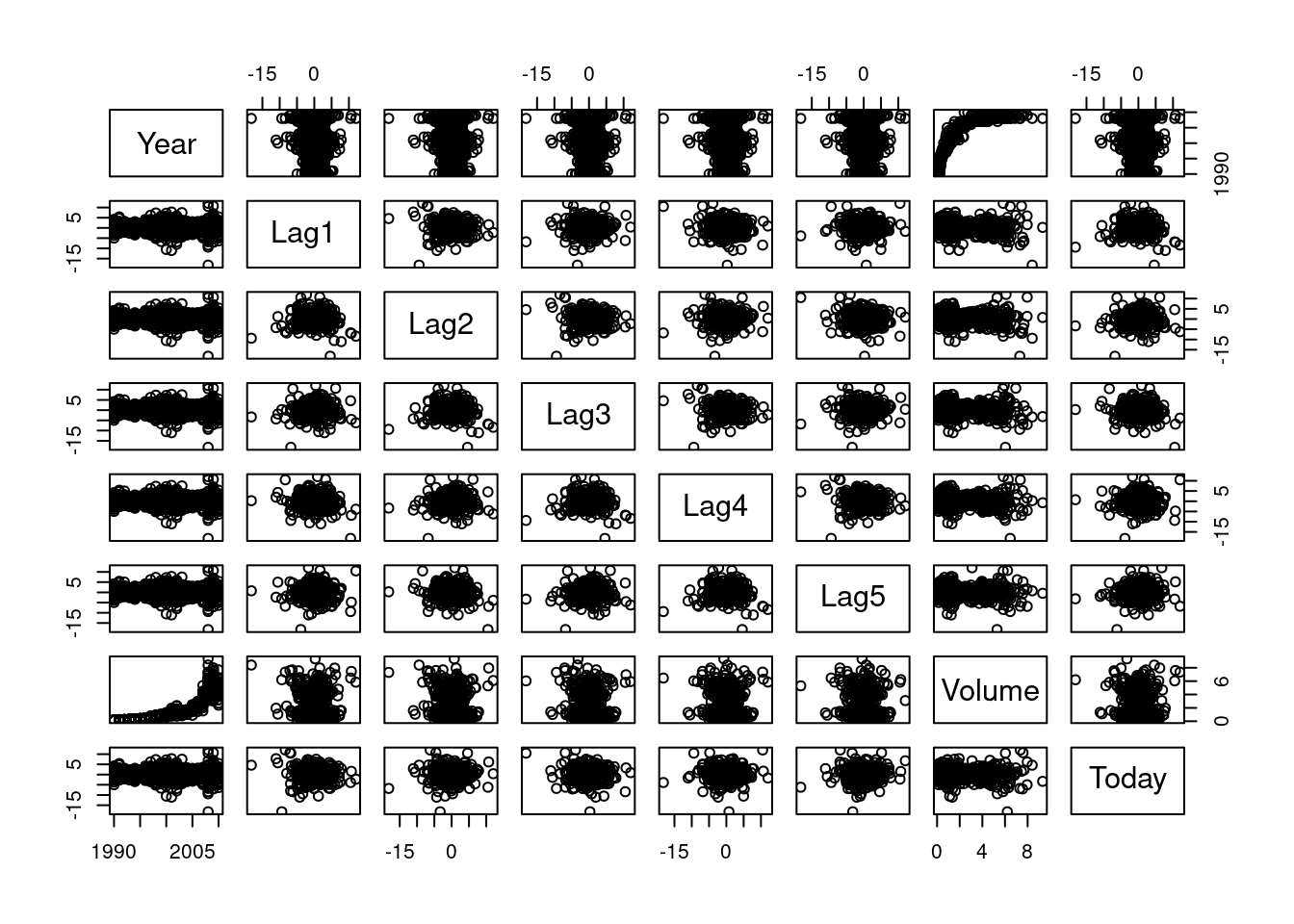
## # scatterplot matrix
pairs(Weekly[,1:8])
# correlation matrix
round(cor(Weekly[,1:8]),2)
## Year Lag1 Lag2 Lag3 Lag4 Lag5 Volume Today
## Year 1.00 -0.03 -0.03 -0.03 -0.03 -0.03 0.84 -0.03
## Lag1 -0.03 1.00 -0.07 0.06 -0.07 -0.01 -0.06 -0.08
## Lag2 -0.03 -0.07 1.00 -0.08 0.06 -0.07 -0.09 0.06
## Lag3 -0.03 0.06 -0.08 1.00 -0.08 0.06 -0.07 -0.07
## Lag4 -0.03 -0.07 0.06 -0.08 1.00 -0.08 -0.06 -0.01
## Lag5 -0.03 -0.01 -0.07 0.06 -0.08 1.00 -0.06 0.01
## Volume 0.84 -0.06 -0.09 -0.07 -0.06 -0.06 1.00 -0.03
## Today -0.03 -0.08 0.06 -0.07 -0.01 0.01 -0.03 1.00# (b) logistic regression
logistic_fit = glm(Direction ~ Lag1+Lag2+Lag3+Lag4+Lag5+Volume, data=Weekly, family=binomial)
summary(logistic_fit)##
## Call:
## glm(formula = Direction ~ Lag1 + Lag2 + Lag3 + Lag4 + Lag5 +
## Volume, family = binomial, data = Weekly)
##
## Coefficients:
## Estimate Std. Error z value Pr(>|z|)
## (Intercept) 0.26686 0.08593 3.106 0.0019 **
## Lag1 -0.04127 0.02641 -1.563 0.1181
## Lag2 0.05844 0.02686 2.175 0.0296 *
## Lag3 -0.01606 0.02666 -0.602 0.5469
## Lag4 -0.02779 0.02646 -1.050 0.2937
## Lag5 -0.01447 0.02638 -0.549 0.5833
## Volume -0.02274 0.03690 -0.616 0.5377
## ---
## Signif. codes: 0 '***' 0.001 '**' 0.01 '*' 0.05 '.' 0.1 ' ' 1
##
## (Dispersion parameter for binomial family taken to be 1)
##
## Null deviance: 1496.2 on 1088 degrees of freedom
## Residual deviance: 1486.4 on 1082 degrees of freedom
## AIC: 1500.4
##
## Number of Fisher Scoring iterations: 4# (c) confusion matrix
logistic_probs = predict(logistic_fit, type="response")
logistic_preds = rep("Down", 1089) # Vector of 1089 "Down" elements.
logistic_preds[logistic_probs>0.5] = "Up" # Change "Down" to up when probability > 0.5.
attach(Weekly)
table(logistic_preds,Direction)## Direction
## logistic_preds Down Up
## Down 54 48
## Up 430 557\[\text{accuracy} = \frac{54 + 557}{54 + 48 + 430 + 557} \approx 0.5611\]
# Training observations from 1990 to 2008.
train = (Year<2009)
# Test observations from 2009 to 2010.
Test = Weekly[!train ,]
Test_Direction= Direction[!train]

# Logistic regression on training set.
logistic_fit2 = glm(Direction ~ Lag2, data=Weekly, family=binomial, subset=train)
# Predictions on the test set.
logistic_probs2 = predict(logistic_fit2,Test, type="response")
logistic_preds2 = rep("Down", 104)
logistic_preds2[logistic_probs2>0.5] = "Up"
# Confusion matrix.
table(logistic_preds2,Test_Direction)
## Test_Direction
## logistic_preds2 Down Up
## Down 9 5
## Up 34 56\[\text{accuracy} = \frac{9 + 56}{9 + 5 + 34 + 56} = 0.625\]
# Using LDA
library("MASS")
lda_fit = lda(Direction ~ Lag2, data=Weekly, subset=train)
#lda_fit
# Predictions on the test set.
lda_pred = predict(lda_fit,Test)
lda_class = lda_pred$class
# Confusion matrix.
table(lda_class,Test_Direction)
## Test_Direction
## lda_class Down Up
## Down 9 5
## Up 34 56\[\text{accuracy} = \frac{9 + 56}{9 + 5 + 34 + 56} = 0.625\]
# Using QDA.
qda_fit = qda(Direction ~ Lag2, data=Weekly, subset=train)
qda_pred = predict(qda_fit,Test)
qda_class = qda_pred$class
table(qda_class,Test_Direction)
## Test_Direction
## qda_class Down Up
## Down 0 0
## Up 43 61# Using KNN
library("class")
set.seed(1)
train_X = Weekly[train,3]
test_X = Weekly[!train,3]
train_direction = Direction[train]
# Changing from vector to matrix by adding dimensions
dim(train_X) = c(985,1)
dim(test_X) = c(104,1)
# Predictions for K=1
knn_pred = knn(train_X, test_X, train_direction, k=1)
table(knn_pred, Test_Direction)## Test_Direction
## knn_pred Down Up
## Down 21 30
## Up 22 31\[\text{accuracy} = \frac{31 + 31}{21 + 30 + 22 + 31} \approx 0.5962\]
- Develop a model to predict whether a given car gets high or low gas milage based on the
Autodata set.
# binary variable for "high" versus "low"
# Dataframe with "Auto" data and empty "mpg01" column
df = Auto
df$mpg01 = NA
median_mpg = median(df$mpg)
# Loop
for(i in 1:dim(df)[1]){
  if (df$mpg[i] > median_mpg){
    df$mpg01[i] = 1
  }else{
    df$mpg01[i] = 0
  }
}
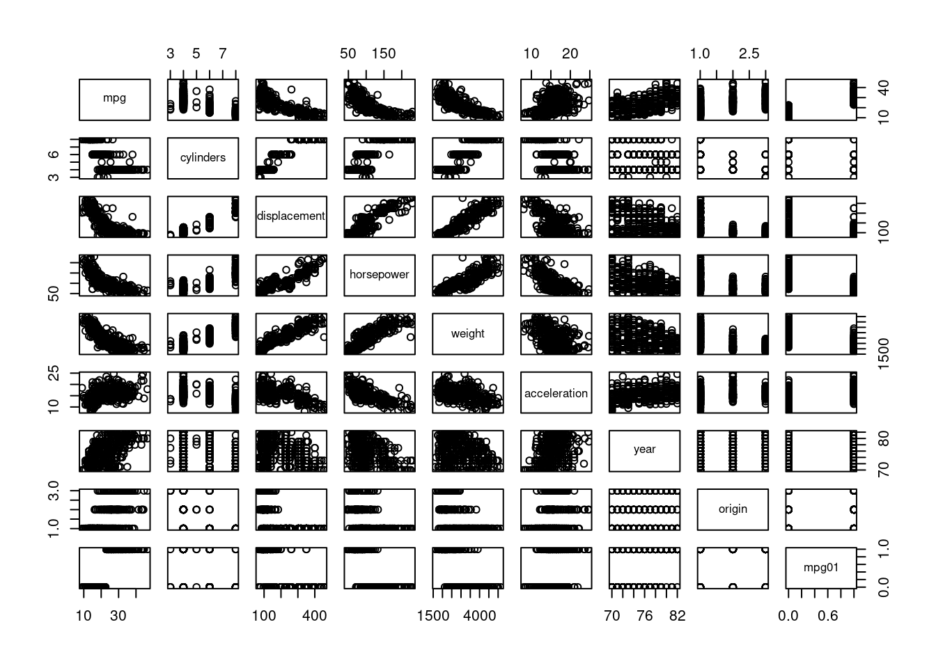
# graphical summary
pairs(df[,c(1:8,10)])
# correlation matrix
round(cor(df[,c(1:8,10)]),2)
## mpg cylinders displacement horsepower weight acceleration year
## mpg 1.00 -0.78 -0.81 -0.78 -0.83 0.42 0.58
## cylinders -0.78 1.00 0.95 0.84 0.90 -0.50 -0.35
## displacement -0.81 0.95 1.00 0.90 0.93 -0.54 -0.37
## horsepower -0.78 0.84 0.90 1.00 0.86 -0.69 -0.42
## weight -0.83 0.90 0.93 0.86 1.00 -0.42 -0.31
## acceleration 0.42 -0.50 -0.54 -0.69 -0.42 1.00 0.29
## year 0.58 -0.35 -0.37 -0.42 -0.31 0.29 1.00
## origin 0.57 -0.57 -0.61 -0.46 -0.59 0.21 0.18
## mpg01 0.84 -0.76 -0.75 -0.67 -0.76 0.35 0.43
## origin mpg01
## mpg 0.57 0.84
## cylinders -0.57 -0.76
## displacement -0.61 -0.75
## horsepower -0.46 -0.67
## weight -0.59 -0.76
## acceleration 0.21 0.35
## year 0.18 0.43
## origin 1.00 0.51
## mpg01 0.51 1.00library('tidyverse')
# split into training and test set
set.seed(123)
df <- df |>
mutate(splitter = sample(c("train", "test"), nrow(df), replace = TRUE))
train2 <- df |> filter(splitter == "train")
test2 <- df |> filter(splitter == "test")# LDA model
lda_fit3 = lda(mpg01 ~ cylinders+displacement+horsepower+weight, data=train2)
# Predictions and confusion matrix
lda_pred3 = predict(lda_fit3,test2)
predictions = lda_pred3$class
actual = test2$mpg01
table(predictions,actual)## actual
## predictions 0 1
## 0 75 5
## 1 19 88\[\text{test error } = \frac{5+19}{75 + 5 + 19 + 88} \approx 0.1284\]
# QDA model
qda_fit2 = qda(mpg01 ~ cylinders+displacement+horsepower+weight, data=train2)
qda_pred2 = predict(qda_fit2,test2)
predictions = qda_pred2$class
table(predictions,actual)
## actual
## predictions 0 1
## 0 82 7
## 1 12 86\[\text{test error } = \frac{7+12}{82 + 7 + 12 + 86} \approx 0.1016\]
# Logistic regression model
logistic_fit5 = glm(mpg01 ~ cylinders+displacement+horsepower+weight, data=train2, family=binomial)
logistic_probs5 = predict(logistic_fit5,test2, type="response")
logistic_preds5 = rep(0, length(test2$mpg01))
logistic_preds5[logistic_probs5>0.5] = 1
table(logistic_preds5,actual)
## actual
## logistic_preds5 0 1
## 0 79 7
## 1 15 86\[\text{test error } = \frac{7+15}{79 + 7 + 15 + 86} \approx 0.1176\]