6.3 Dimension Reduction Methods
- Transform predictors before use.
- \(Z_1, Z_2, ..., Z_M\) represent \(M < p\) linear combinations of original p predictors.
\[Z_m = \sum_{j=1}^p{\phi_{jm}X_j}\]
- Linear regression using the transformed predictors can “often” outperform linear regression using the original predictors.
The Math
\[Z_m = \sum_{j=1}^p{\phi_{jm}X_j}\] \[y_i = \theta_0 + \sum_{m=1}^M{\theta_mz_{im} + \epsilon_i}, i = 1, ..., n\] \[\sum_{m=1}^M{\theta_mz_{im}} = \sum_{m=1}^M{\theta_m}\sum_{j=1}^p{\phi_{jm}x_ij}\] \[\sum_{m=1}^M{\theta_mz_{im}} = \sum_{j=1}^p\sum_{m=1}^M{\theta_m\phi_{jm}x_ij}\] \[\sum_{m=1}^M{\theta_mz_{im}} = \sum_{j=1}^p{\beta_jx_ij}\] \[\beta_j = \sum_{m=1}^M{\theta_m\phi_{jm}}\]
- Dimension reduction constrains \(\beta_j\)
- Can increase bias, but (significantly) reduce variance when \(M \ll p\)
Principal Components Regression
- PCA chooses \(\phi\)s to capture as much variance as possible.
- Will be discussed in more detail in Chapter 12.
- First principal component = direction of the data is that along which the observations vary the most.
- Second principal component = orthogonal to 1st, capture next most variation
- Etc
- Create new ‘predictors’ that are more independent and potentially fewer, which improves test MSE, but note that this doe not help improve interpretability (all \(p\) predictors are still involved.)
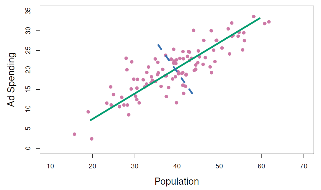
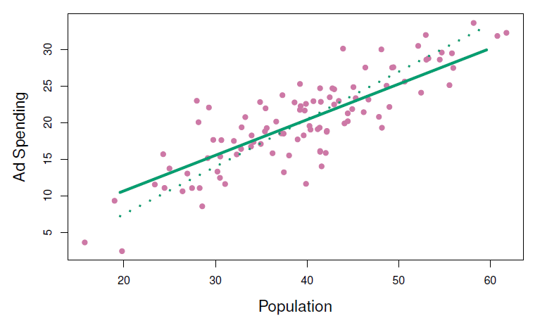
Figure 6.14
Principal Components Regression
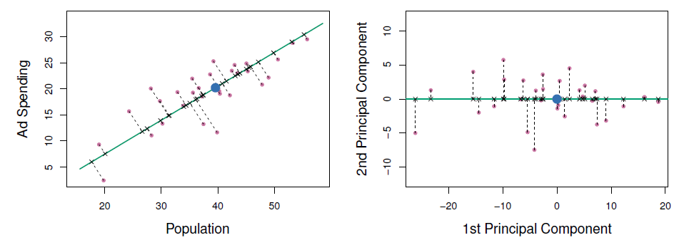
Figure 6.15
\[Z_1 = 0.839 \times (\mathrm{pop} - \overline{\mathrm{pop}}) + 0.544 \times (\mathrm{ad} - \overline{\mathrm{ad}})\]
Principal Components Regression
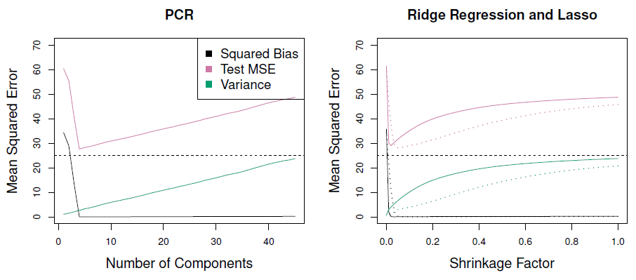
Figure 6.19
- Mitigate overfitting by reducing number of variables.
- Assume that the directions in which \(X\) shows the most variation are the directions associated with variation in \(Y\).
- When assumption is true, PCR can do very well.
- Note: PCR isn’t feature selection, since PCs depend on all \(p\)s.
- More like ridge than lasso.
- Best to standardize variables before PCR.
Example
In the figures below, PCR fits on simulated data are shown. Both were generated usign n=50 observations and p = 45 predictors. First data set response uses all the predictors, while in seond it uses only two. PCR improves over OLS at least in the first case. In the second case the improvement is modest, perhaps because the assumption that the directions of maximal variations in predictors doesnt correlate well with variations in the response as assumed by PCR.
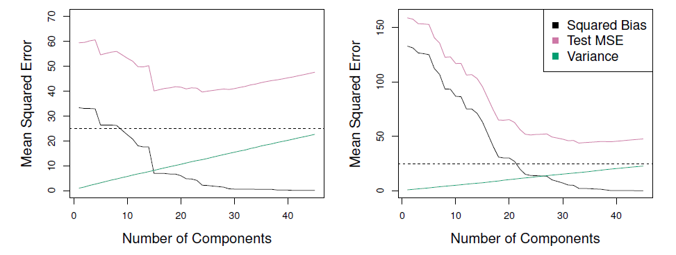
Figure 6.18
- When variation in \(X\) isn’t strongly correlated with variation in \(Y\), PCR isn’t as effective.