10.2 Single Layer Neural Network

Let’s consider a dataset made of \(p\) predictors

\[X=(X_1,X_2,X_3,...,X_p)\]

and build a non linear function \(f(X)\) to predict a response \(Y\).

\[f(X)=\beta_0+\sum_{k=1}^K{\beta_kh_k(X)}\]

where \(h_k(X)\) is the expression of the hidden layers, a transformation of the input, named as the \(A_k\) function of \(X\) with \(K\) activation, \(k=1,...,K\), which are not directly observed.

\[A_k=h_k(X)\] and identify the activation: a non linear transformation of a linear function \(g(z)\)

\[A_k=h_k(X)=g(z)\]

\[A_k=h_k(X)=g(w_{k0}+\sum_{j=1}^p{w_{kj}X_j})\] to obtain an output layer which is a linear model that uses these activations \(A_k\) as inputs, resulting in a function \(f(X)\).

\[f(X)=\beta_0+\sum_{k=1}^K{\beta_kA_k}\] aech \(A_k\) is a different transformation of \(h_k(X)\)

\(\beta_0,...,B_K\) and \(w_{1,0},...,w_{K,p}\) need to be estimated from data.

What about the activation function \(g(z)\)? There are various options, but the most used ones are:

1. sigmoid

\[g(z)=\frac{e^z}{1+e^z}\]

2. ReLU rectified linear unit

\[g(z)=(z)_+=\left\{ \begin{array}{ll} 0 & \mbox{if z<0};\\ 1 & \mbox{otherwise}.\end{array}\right.\]

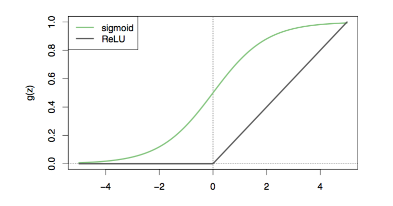
Figure 10.1: Activation functions - Chap 10

This is the structure of a single layer neural network. Here we can see the layer inputs, the hidden layers and the output layer.

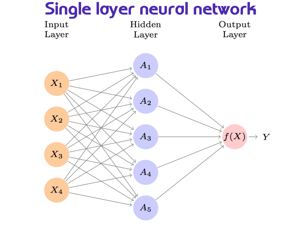
Figure 10.2: Single layer neural network - Chap 10

In this example, we see deep learning applied to dosage/efficacy study, the model parameters with the activation function in the middle.

The parameters can be retrieved with backpropagation which optimizes weights for coefficients \(w_{kj}\) and biases for the intercepts \(w_{k0}\). We will see about that later on this notes. For now we suppose to know what is the value of the parameters, and we investigate the calculation of the deep learning model.

\[f(X)=\beta_0+\sum_{k=1}^K{\beta_kg(w_{k0}+\sum_{wkj}^p{X_j})}\]

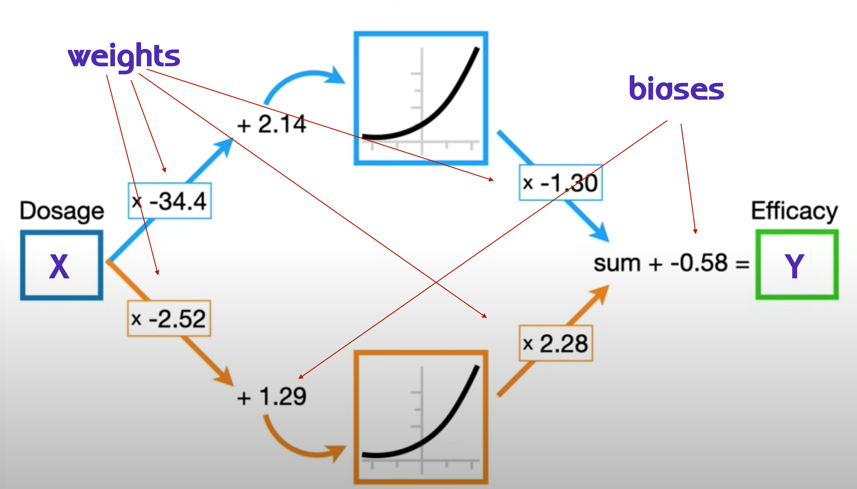
Figure 10.3: Neural network Pt.1 Inside the black box - Youtube video

Neural network Pt.1 Inside the black box

This is from the book pg.406, and you can see all the passages for calculating the estimated \(f(X)\) supposing that we know the value of the parameters.

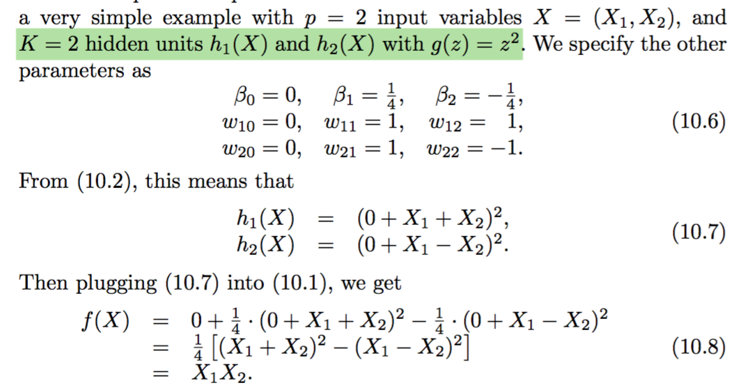
Figure 10.4: Neural network model fit calculation - Chap 10

Fitting a quantitative neural network to estimate the unknown parameters \(w_{kj}\) and \(\beta_{k}\) requires the squared-error loss function to be minimum.

Mean squared-error:

\[min\sum{i=1}^n{(y_i-f(x_i))^2}\]

Or to train a qualitative neural network is to minimizing the negative multinomial log-likelihood or the \[cross-entrophy\]. We see this explained in the multilayer neural network section.

Min of the negative multinomial log-likelyhood:

\[-\sum_{i=1}^n{\sum_{m=0}^K{y_{im}log(f_m(x_i))}}\]

As deep learnig models have the ability to fit a good squiggle lines to data, the estimated parameters can be applied to a special softmax function:

\[f_{m}=Pr(Y=m|X)=\frac{e^{Z_m}}{\sum_{k=0}^K{e^{Z_k}}}\]