4.11 Poisson distribution

A count response variable \(Y\) (which takes on non-negative integer values) can be modeled using the Poisson distribution, where the probability that \(Y\) takes on a given count value \(k\) can be calculated as:

\(Pr(Y = k) = \frac{e^{-\lambda}\lambda^k}{k!}\) for \(k\) = 0, 1, 2, …

where \(\lambda\) represents both the expected value (mean) and variance of \(Y\):

\(Y = E(Y) = Var(Y)\)

=> “[I]f \(Y\) follows the Poisson distribution, then the larger the mean of \(Y\), the larger its variance.”

par(mfrow = c(2,2))
lambda <- c(1:4)
k <- c(0:10)
for (lam in lambda) {
  Prk <- (exp(-lam)*lam^k)/factorial(k)
  plot(k, Prk, type = 'b', ylim = c(0, 0.4), main = paste("lambda =", lam))
}

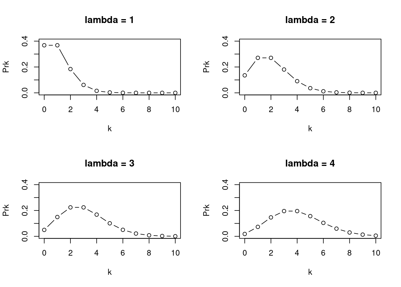
Figure 4.15: Plots of Poisson Distributions with different lambda values, showing how variance increases with increasing lambda. Note all values are non-negative integer values, suitable for modelling counts, k.