12.4 Proportion of variance explained

First we look at the variance

names(USArrests_pca)

## [1] "sdev"     "rotation" "center"   "scale"    "x"

pr.var <- USArrests_pca$sdev^2
pr.var

## [1] 2.4802416 0.9897652 0.3565632 0.1734301

Proportion of variance explained by each principal component:

pve <- pr.var / sum(pr.var)
pve

## [1] 0.62006039 0.24744129 0.08914080 0.04335752

par(mfrow = c(1, 2))
plot(pve, xlab = "Principal Component",
ylab = "Proportion of Variance Explained", ylim = c(0, 1),
type = "b")
plot(cumsum(pve), xlab = "Principal Component",
ylab = "Cumulative Proportion of Variance Explained", ylim = c(0, 1), type = "b")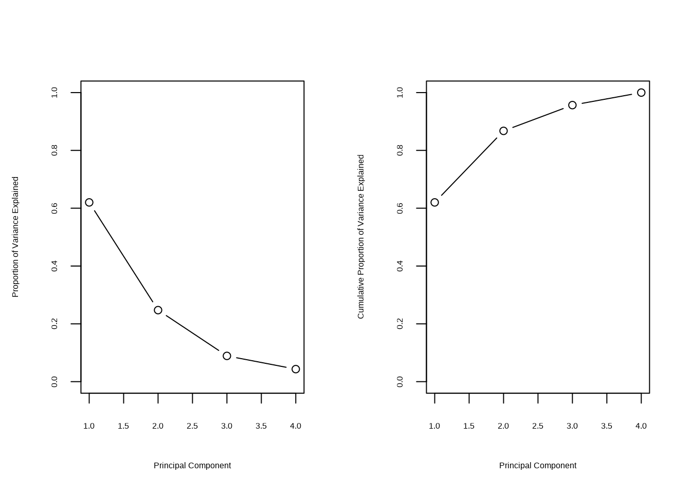

X <- data.matrix(scale(USArrests[,-1])) 
pcob <- prcomp(X)
summary(pcob)

## Importance of components:
##                           PC1    PC2     PC3     PC4
## Standard deviation     1.5749 0.9949 0.59713 0.41645
## Proportion of Variance 0.6201 0.2474 0.08914 0.04336
## Cumulative Proportion  0.6201 0.8675 0.95664 1.00000