7.2 Splines
A linear spline is a piecewise linear polynomial continuous at each knot.
We can represent this model as
\[ y_i = \beta_0 + \beta_1b_1(x_i) + \beta_2b_2(x_i) + · · · + \beta_{K+1}b_{K+1}(x_i) + \epsilon_i \] where the \(b_k\) are basis functions.
###

fit <- lm(wage ~ bs(age, knots = c(25, 40, 60)), data = Wage)
agelims <- range(Wage$age)
age.grid <- seq(from = agelims[1], to = agelims[2])
pred <- predict(fit, newdata = list(age = age.grid), se = T)
plot(Wage$age, Wage$wage, col = "gray")
title("Poly B-Spline Basis w 3 knots and Natural Cubic Spline")
lines(age.grid, pred$fit, lwd = 2)
lines(age.grid, pred$fit + 2 * pred$se, lty = "dashed")
lines(age.grid, pred$fit - 2 * pred$se, lty = "dashed")
###
fit2 <- lm(wage ~ ns(age, df = 4), data = Wage)
pred2 <- predict(fit2, newdata = list(age = age.grid),
     se = T)
lines(age.grid, pred2$fit, col = "red", lwd = 2)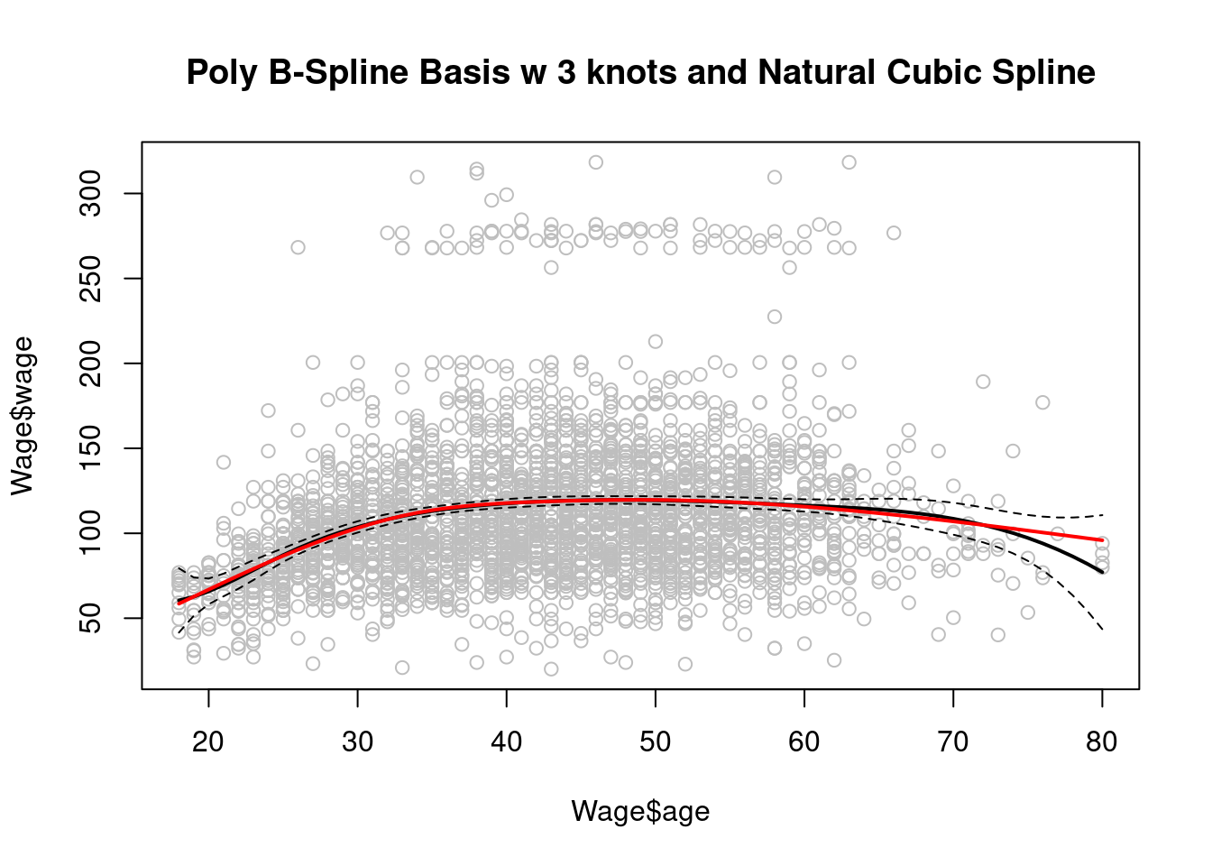
Cubic Splines
A cubic spline is a piecewise cubic polynomial with continuous derivatives up to order 2 at each knot.
- To apply a cubic spline, the knot locations have to be defined. Intuitively, one might locate them at the quartile breaks or at range boundaries that are significant for the data domain.
Natural Cubic Splines
A natural cubic spline extrapolates linearly beyond the boundary knots. This adds 4 = 2 × 2 extra constraints, and allows us to put more internal knots for the same degrees of freedom as a regular cubic spline above.
Fitting natural splines is easy. A cubic spline with K knots has K + 4 parameters or degrees of freedom. A natural spline with K knots has K degrees of freedom.
The result is often a simpler, smoother, more generalizable function with less bias.
Smoothing Splines
The solution is a natural cubic spline, with a knot at every unique value of \(x_i\). A roughness penalty controls the roughness via \(\lambda\).
Smoothing splines avoid the knot-selection issue mathematically, leaving a single λ to be chosen.
in the R function
smooth.splinethe degrees of freedom is often specified, not the λsmooth.splinehas a built-in cross-validation function to choose a suitable DF automatically, as ordinary leave-one-out (TRUE) or ‘generalized’ cross-validation (GCV) when FALSE. The ‘generalized’ cross-validation method GCV technique will work best when there are duplicated points in x.
###
plot(Wage$age, Wage$wage, xlim = agelims, cex = .5, col = "darkgrey")
title("Smoothing Spline")

fit <- smooth.spline(Wage$age, Wage$wage, df = 16)
fit2 <- smooth.spline(Wage$age, Wage$wage, cv = TRUE)
## Warning in smooth.spline(Wage$age, Wage$wage, cv = TRUE): cross-validation with
## non-unique 'x' values seems doubtfullines(fit, col = "red", lwd = 2)
lines(fit2, col = "blue", lwd = 2)
legend("topright", legend = c("16 DF", "6.8 DF"),
col = c("red", "blue"), lty = 1, lwd = 2, cex = .8)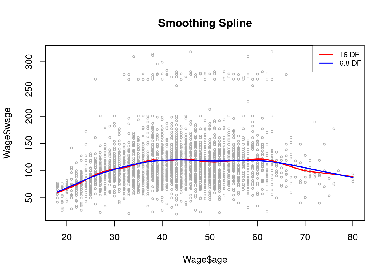
Local Regression
Local regression is a slightly different approach for fitting which involves computing the fit at a target point \(x_i\) using only nearby observations.
The loess fit yields a walk with a span parameter to arrive at a spline fit.
###
plot(Wage$age, Wage$wage, xlim = agelims, cex = .5, col = "darkgrey")
title("Local Regression")

fit <- loess(wage ~ age, span = .2, data = Wage)
fit2 <- loess(wage ~ age, span = .5, data = Wage)
lines(age.grid, predict(fit, data.frame(age = age.grid)),
    col = "red", lwd = 2)
lines(age.grid, predict(fit2, data.frame(age = age.grid)),
    col = "blue", lwd = 2)
legend("topright", legend = c("Span = 0.2", "Span = 0.5"),
    col = c("red", "blue"), lty = 1, lwd = 2, cex = .8)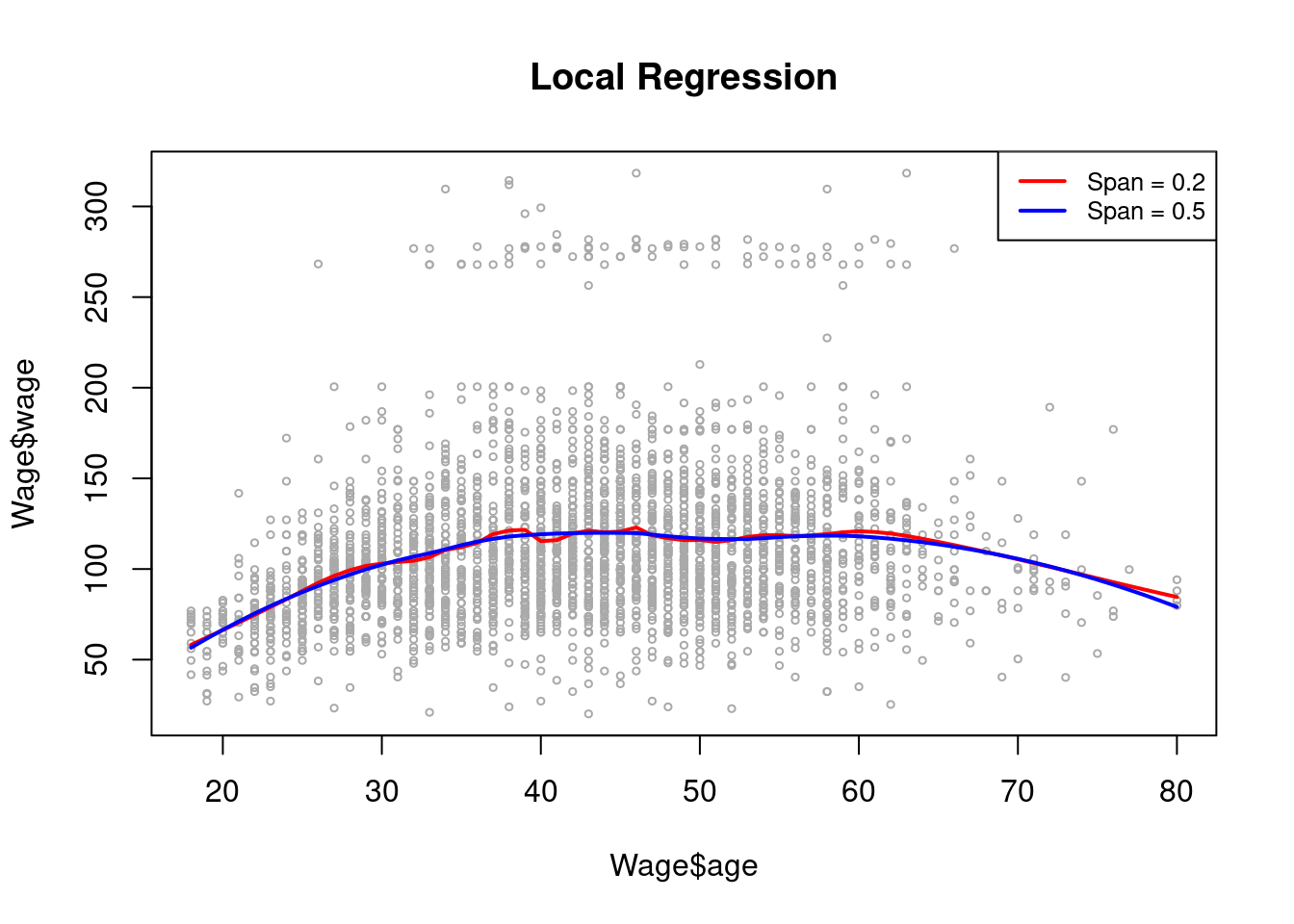
So far, every example model has shown one independent variable and one dependent variable. Much more utility comes when these techniques are generalized broadly for many independent variables.
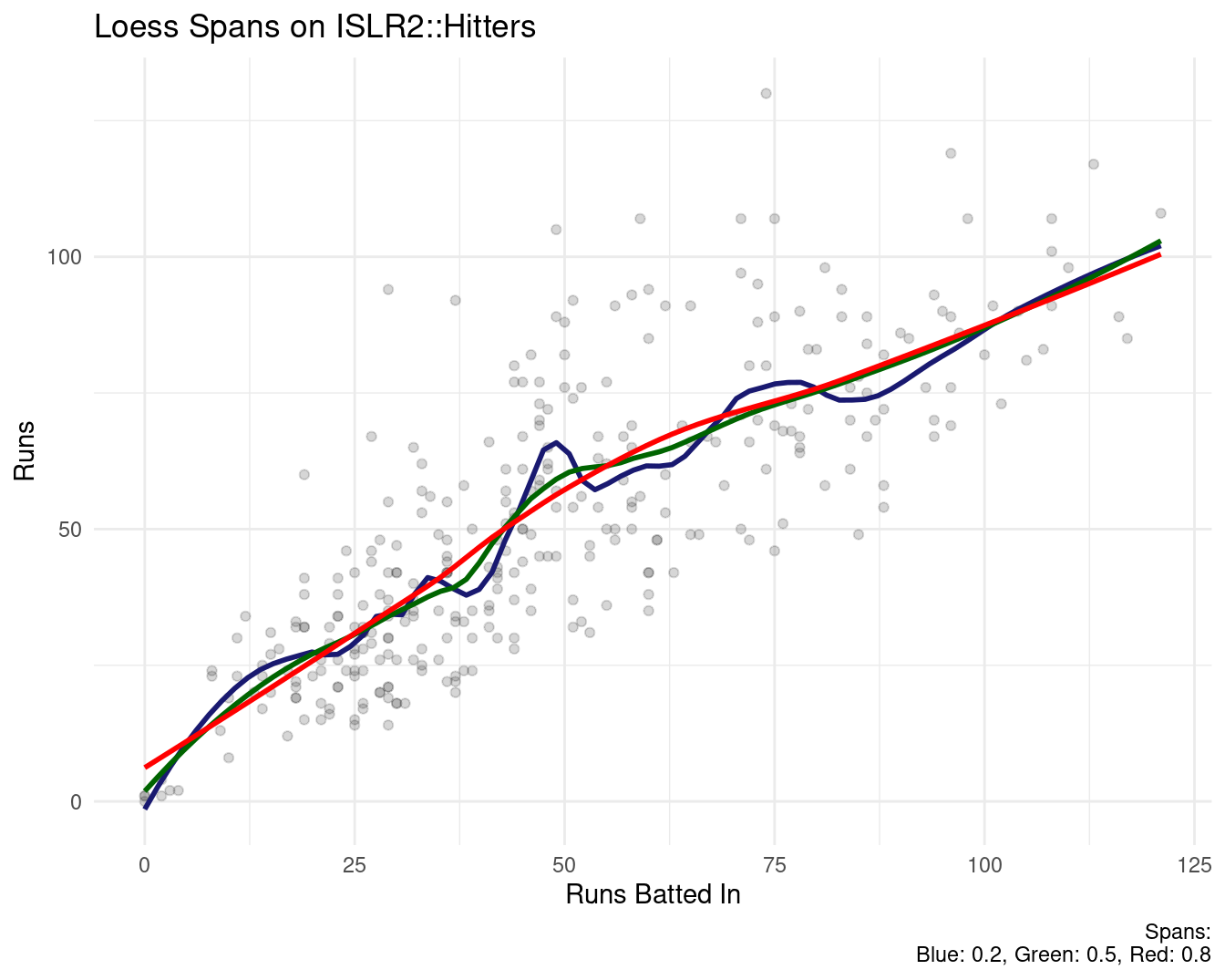
A side note - normal ggplot geom_smooth for small datasets applies the loess method.
as_tibble(ISLR2::Hitters) %>%
  ggplot(aes(RBI, Runs)) +
  geom_point(alpha = 0.2, color = "gray20") +
  stat_smooth(method = "loess", span = 0.2, color = "midnightblue", se = F) +
  stat_smooth(method = "loess", span = 0.5, color = "darkgreen", se = F) +
  stat_smooth(method = "loess", span = 0.8, color = "red", se = F) +
  labs(title = "Loess Spans on ISLR2::Hitters",
       x = "Runs Batted In", y = "Runs",
       caption = "Spans:\nBlue: 0.2, Green: 0.5, Red: 0.8") +
  theme_minimal()
## `geom_smooth()` using formula = 'y ~ x'
## `geom_smooth()` using formula = 'y ~ x'
## `geom_smooth()` using formula = 'y ~ x'