10.10 Case Study: RNN - Time Series
The idea is to extract many short mini-series of input sequences \(X=X_1,X_2,...,X_L\) with a predefined length L (called the lag) and a corresponding target Y.
The target Y is the value of the log volume \(v_t\) at a single timepoint \(t\), and the input sequence X is the series of 3-vectors \({X_ℓ}^L\) each consisting of the three measurements log volume, DJ return and log volatility from day \(t−L, t−L+1, ... t−1\). Each value of time \(t\) makes a separate \((X,Y)\) pair, for \(t\) running from \(L+1\) to \(T\).
10.10.0.0.1 Autoregression
The RNN fit has much in common with a traditional autoregression (AR) linear model. They both use the same response \(Y\) and input sequences \(X\) of length \(L=5\) and dimension \(p=3\) in this case.
The RNN processes this sequence from left to right with the same weights \(W\) (for the input layer), while the AR model simply treats all L elements of the sequence equally as a vector of \(L×p\) predictors, a process called flattening in the neural network literature.
The RNN also includes the hidden layer activations \(A\) which transfer information along the sequence, and introduces additional non-linearity.
library(tidyverse)
library(ISLR2)
NYSE%>%head
## date day_of_week DJ_return log_volume log_volatility train
## 1 1962-12-03 mon -0.004461 0.032573 -13.12740 TRUE
## 2 1962-12-04 tues 0.007813 0.346202 -11.74930 TRUE
## 3 1962-12-05 wed 0.003845 0.525306 -11.66561 TRUE
## 4 1962-12-06 thur -0.003462 0.210182 -11.62677 TRUE
## 5 1962-12-07 fri 0.000568 0.044187 -11.72813 TRUE
## 6 1962-12-10 mon -0.010824 0.133246 -10.87253 TRUExdata <- data.matrix(
NYSE[, c("DJ_return",
"log_volume",
"log_volatility")]
)
xdata %>% head## DJ_return log_volume log_volatility
## [1,] -0.004461 0.032573 -13.12740
## [2,] 0.007813 0.346202 -11.74930
## [3,] 0.003845 0.525306 -11.66561
## [4,] -0.003462 0.210182 -11.62677
## [5,] 0.000568 0.044187 -11.72813
## [6,] -0.010824 0.133246 -10.87253istrain <- NYSE[, "train"]
xdata <- scale(xdata)Make a function to create lagged versions of the three time series.
lagm <- function(x, k = 1) {
  n <- nrow(x)
  pad <- matrix(NA, k, ncol(x))
  rbind(pad, x[1:(n - k), ])
}
Apply the lags:
arframe <- data.frame(log_volume = xdata[, "log_volume"],
   L1 = lagm(xdata, 1), L2 = lagm(xdata, 2),
   L3 = lagm(xdata, 3), L4 = lagm(xdata, 4),
   L5 = lagm(xdata, 5)
 )

arframe %>% head(3,3)
## log_volume L1.DJ_return L1.log_volume L1.log_volatility L2.DJ_return
## 1 0.1750605 NA NA NA NA
## 2 1.5171653 -0.5497779 0.1750605 -4.356718 NA
## 3 2.2836006 0.9051251 1.5171653 -2.528849 -0.5497779
## L2.log_volume L2.log_volatility L3.DJ_return L3.log_volume L3.log_volatility
## 1 NA NA NA NA NA
## 2 NA NA NA NA NA
## 3 0.1750605 -4.356718 NA NA NA
## L4.DJ_return L4.log_volume L4.log_volatility L5.DJ_return L5.log_volume
## 1 NA NA NA NA NA
## 2 NA NA NA NA NA
## 3 NA NA NA NA NA
## L5.log_volatility
## 1 NA
## 2 NA
## 3 NAarframe <- arframe[-(1:5), ]
istrain <- istrain[-(1:5)]10.10.0.1 Linear AR model
The “AR” stands for autoregression, indicating that the model uses the dependent relationship between current data and its past values.
Fit the linear AR model to the training data using lm(), and predict on the test data.
arfit <- lm(log_volume ~ .,
            data = arframe[istrain, ])

summary(arfit)
##
## Call:
## lm(formula = log_volume ~ ., data = arframe[istrain, ])
##
## Residuals:
## Min 1Q Median 3Q Max
## -4.1733 -0.3955 -0.0237 0.3831 4.8322
##
## Coefficients:
## Estimate Std. Error t value Pr(>|t|)
## (Intercept) -0.006254 0.010067 -0.621 0.534500
## L1.DJ_return 0.094605 0.010904 8.676 < 2e-16 ***
## L1.log_volume 0.507492 0.016313 31.109 < 2e-16 ***
## L1.log_volatility 0.579946 0.054138 10.712 < 2e-16 ***
## L2.DJ_return -0.027994 0.011142 -2.512 0.012025 *
## L2.log_volume 0.041132 0.018238 2.255 0.024165 *
## L2.log_volatility -0.937324 0.075844 -12.359 < 2e-16 ***
## L3.DJ_return 0.037671 0.011133 3.384 0.000722 ***
## L3.log_volume 0.074583 0.018097 4.121 3.84e-05 ***
## L3.log_volatility 0.219544 0.077237 2.842 0.004498 **
## L4.DJ_return -0.005442 0.011134 -0.489 0.625051
## L4.log_volume 0.119635 0.017787 6.726 1.98e-11 ***
## L4.log_volatility -0.035429 0.076926 -0.461 0.645135
## L5.DJ_return -0.030128 0.010846 -2.778 0.005496 **
## L5.log_volume 0.098076 0.015527 6.317 2.95e-10 ***
## L5.log_volatility 0.152220 0.054215 2.808 0.005012 **
## ---
## Signif. codes: 0 '***' 0.001 '**' 0.01 '*' 0.05 '.' 0.1 ' ' 1
##
## Residual standard error: 0.6484 on 4260 degrees of freedom
## Multiple R-squared: 0.5707, Adjusted R-squared: 0.5692
## F-statistic: 377.6 on 15 and 4260 DF, p-value: < 2.2e-16arpred <- predict(arfit, arframe[!istrain, ])full_arpred <- data.frame(pred=arpred,
log_volume=arframe[!istrain, "log_volume"])
full_arpred %>%
ggplot(aes(x=log_volume,y=pred))+
geom_point(alpha=0.5)+
geom_smooth(method = "lm")## `geom_smooth()` using formula = 'y ~ x'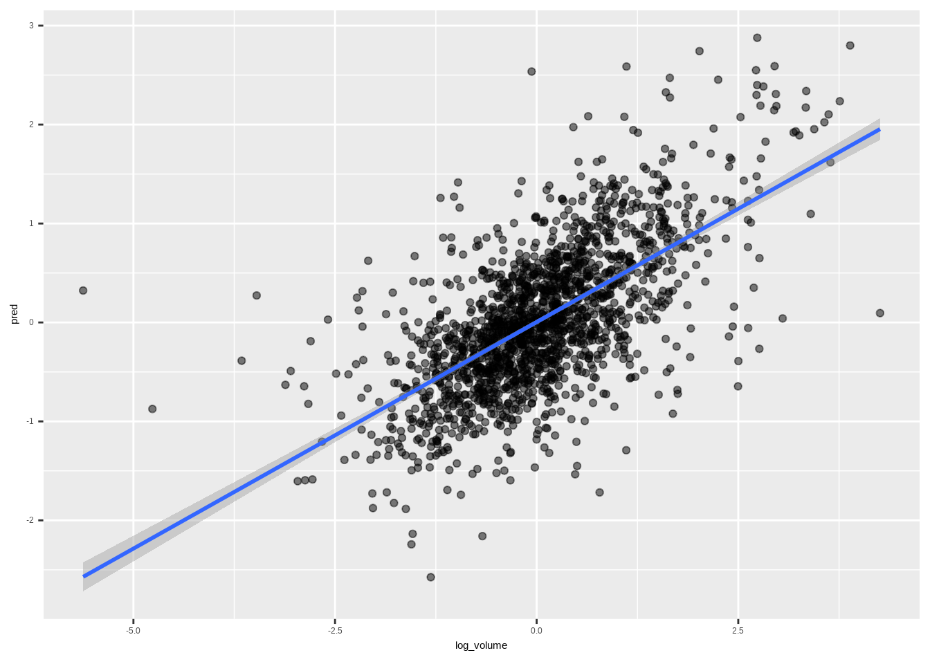
10.10.0.2 Add day_of_week in the model
Re-fit this model, including the factor variable day_of_week.
arframed <- data.frame(day = NYSE[-(1:5), "day_of_week"], arframe)

arframed%>%head
## day log_volume L1.DJ_return L1.log_volume L1.log_volatility L2.DJ_return
## 6 mon 0.60586798 0.046336436 0.22476000 -2.500763 -0.431361080
## 7 tues -0.01365982 -1.304018428 0.60586798 -1.365915 0.046336436
## 8 wed 0.04254846 -0.006293266 -0.01365982 -1.505543 -1.304018428
## 9 thur -0.41980156 0.377050100 0.04254846 -1.551386 -0.006293266
## 10 fri -0.55601945 -0.411684210 -0.41980156 -1.597475 0.377050100
## 11 mon -0.17673016 0.508742889 -0.55601945 -1.564257 -0.411684210
## L2.log_volume L2.log_volatility L3.DJ_return L3.log_volume L3.log_volatility
## 6 0.93509830 -2.366325 0.434776822 2.28360065 -2.417837
## 7 0.22476000 -2.500763 -0.431361080 0.93509830 -2.366325
## 8 0.60586798 -1.365915 0.046336436 0.22476000 -2.500763
## 9 -0.01365982 -1.505543 -1.304018428 0.60586798 -1.365915
## 10 0.04254846 -1.551386 -0.006293266 -0.01365982 -1.505543
## 11 -0.41980156 -1.597475 0.377050100 0.04254846 -1.551386
## L4.DJ_return L4.log_volume L4.log_volatility L5.DJ_return L5.log_volume
## 6 0.905125145 1.51716533 -2.528849 -0.54977791 0.1750605
## 7 0.434776822 2.28360065 -2.417837 0.90512515 1.5171653
## 8 -0.431361080 0.93509830 -2.366325 0.43477682 2.2836006
## 9 0.046336436 0.22476000 -2.500763 -0.43136108 0.9350983
## 10 -1.304018428 0.60586798 -1.365915 0.04633644 0.2247600
## 11 -0.006293266 -0.01365982 -1.505543 -1.30401843 0.6058680
## L5.log_volatility
## 6 -4.356718
## 7 -2.528849
## 8 -2.417837
## 9 -2.366325
## 10 -2.500763
## 11 -1.365915arfitd <- lm(log_volume ~ .,
data = arframed[istrain, ])arpredd <- predict(arfitd, arframed[!istrain, ])full_arpredd <- data.frame(pred=arpredd,
log_volume=arframed[!istrain, "log_volume"])
full_arpred %>%
mutate(type="arpred")%>%
rbind(full_arpredd%>%mutate(type="arpredd")) %>%
ggplot(aes(x=log_volume,y=pred,group=type,color=type))+
geom_point(alpha=0.5)+
geom_smooth(method = "lm")+
scale_color_viridis_d()+
theme_bw()## `geom_smooth()` using formula = 'y ~ x'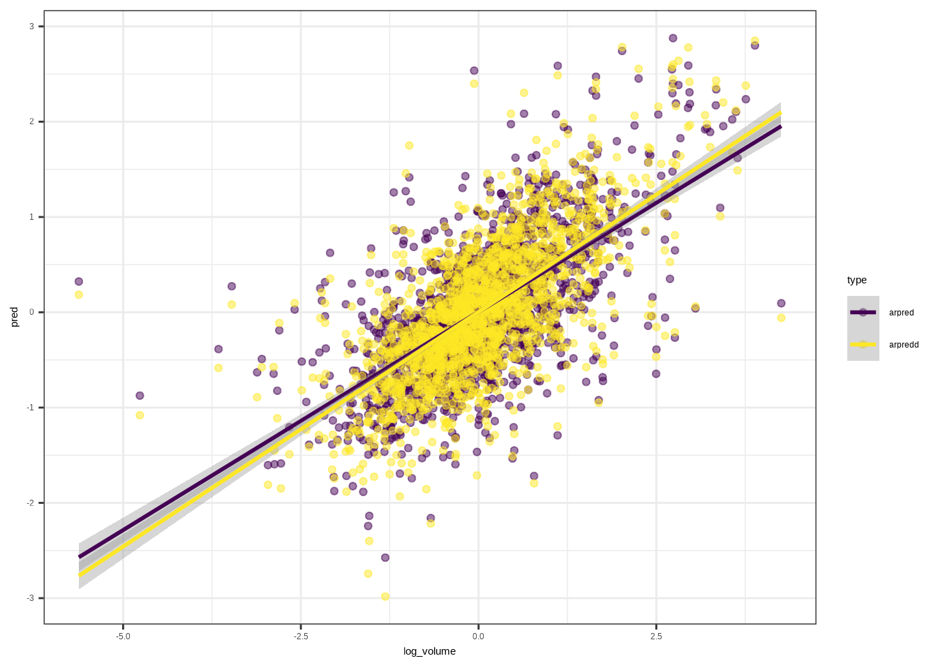
\[R^2(\text{+day of week})=0.4598616\]
1 - mean((arpredd - arframe[!istrain, "log_volume"])^2) / V0## [1] 0.459861610.10.0.3 Preprocessing
To fit the RNN reshape the data sequencing L=5 feature vectors \(X=(Xℓ)_1^L\) for each observation.
(book source (10.20) on page 428)
These are lagged versions of the time series going back L time points.
Preprocessing step transoforming data into a matrix.
n <- nrow(arframe)
xrnn <- data.matrix(arframe[, -1])
xrnn <- array(xrnn, c(n, 3, 5))
xrnn <- xrnn[,, 5:1]
xrnn <- aperm(xrnn, c(1, 3, 2))dim(xrnn)## [1] 6046 5 310.10.0.4 RNN Model
To start using Keras, follow this order:
library(reticulate)
virtualenv_create("r-reticulate", python = path_to_python)
library(tensorflow)
use_virtualenv("r-reticulate")library(keras)Set the model specidfications:
model <- keras_model_sequential() %>%
  layer_simple_rnn(
    units = 12,
    input_shape = list(5, 3),
    dropout = 0.1,
    recurrent_dropout = 0.1
  ) %>%
  layer_dense(units = 1)
model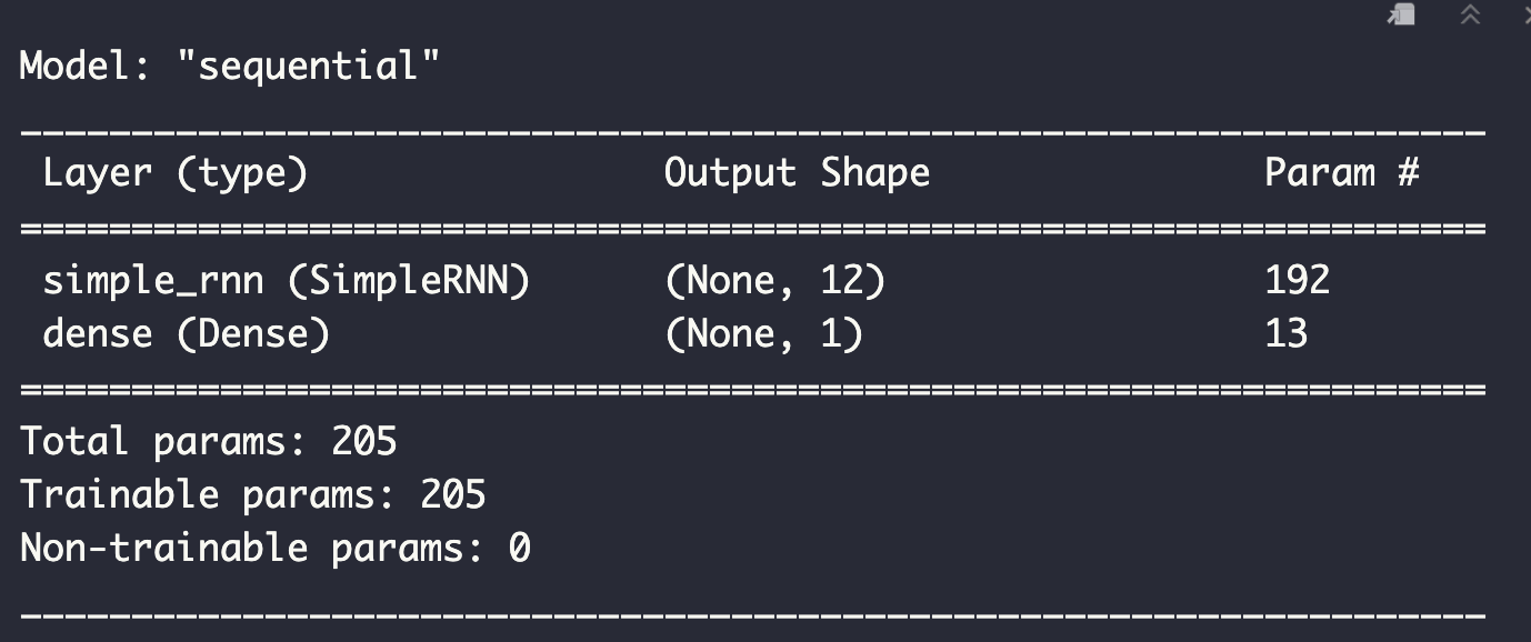
Compile the model with adding specification of parameters optimization:
model %>%
  compile(optimizer = optimizer_rmsprop(),
    loss = "mse")
10.10.0.5 History (RNN model fit)
history <- model %>%
  fit(
    # training set
    xrnn[istrain,, ],
    arframe[istrain, "log_volume"],
    batch_size = 64,
    epochs = 200,
    # testing set
    validation_data = list(xrnn[!istrain,, ],
                           arframe[!istrain, "log_volume"])
)knitr::include_graphics("images/10_history_ts_plot.png")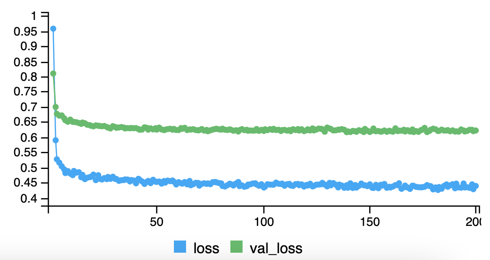
kpred <- predict(model, xrnn[!istrain,, ])This value varies if the model runs more than one time on the same training set, for reproducibility the history need to be run anytime before the predict() function. This assures that the \(R^2\) calculation below releases consistent results.
\[R^2(\text{keras})=0.4102655\]
1 - mean((kpred - arframe[!istrain, "log_volume"])^2) / V010.10.0.6 Model 2
Set a nonlinear AR model extracting the model matrix x from arframed, which includes the day_of_week variable.
x <- model.matrix(log_volume ~ . - 1,
                  data = arframed)

colnames(x)
## [1] "dayfri" "daymon" "daythur"
## [4] "daytues" "daywed" "L1.DJ_return"
## [7] "L1.log_volume" "L1.log_volatility" "L2.DJ_return"
## [10] "L2.log_volume" "L2.log_volatility" "L3.DJ_return"
## [13] "L3.log_volume" "L3.log_volatility" "L4.DJ_return"
## [16] "L4.log_volume" "L4.log_volatility" "L5.DJ_return"
## [19] "L5.log_volume" "L5.log_volatility"arnnd <- keras_model_sequential() %>%
layer_dense(units = 32, activation = 'relu',
input_shape = ncol(x)) %>%
layer_dropout(rate = 0.5) %>%
layer_dense(units = 1)arnnd %>%
compile(loss = "mse",
optimizer = optimizer_rmsprop())10.10.0.7 History 2 (RNN model2 fit)
history2 <- arnnd %>%
  fit(
    x[istrain, ], arframe[istrain, "log_volume"],
    epochs = 100,
    batch_size = 32,
    validation_data =
      list(x[!istrain, ], arframe[!istrain, "log_volume"])
)knitr::include_graphics("images/10_history2_ts_plot.png")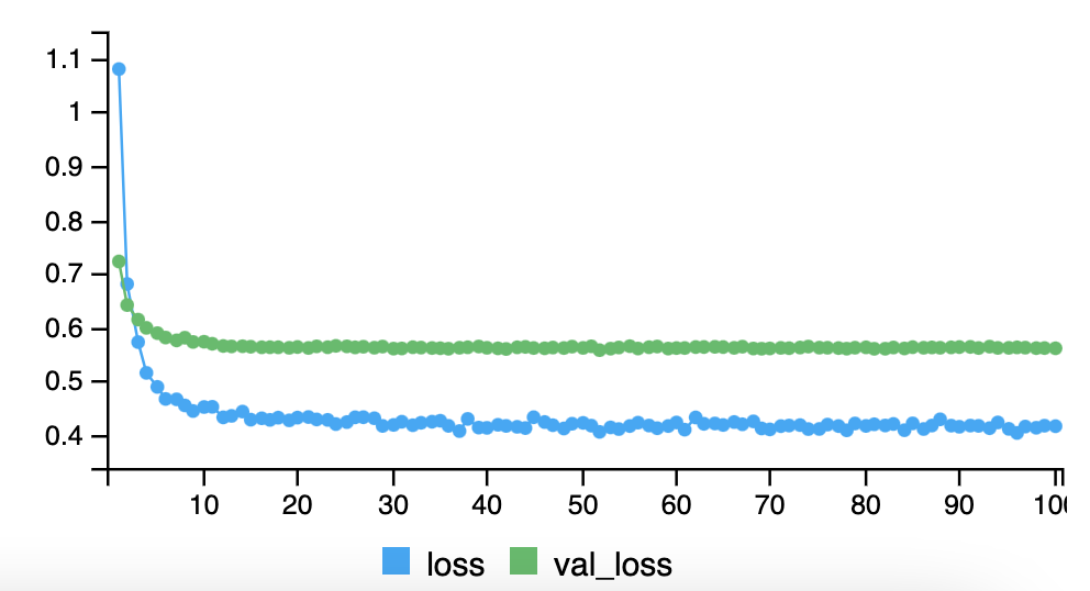
npred <- predict(arnnd, x[!istrain, ])\[R^2=0.4675589\]
1 - mean((arframe[!istrain, "log_volume"] - npred)^2) / V0