Variation
- variation: the tendency of values of a variable to change between measurements.
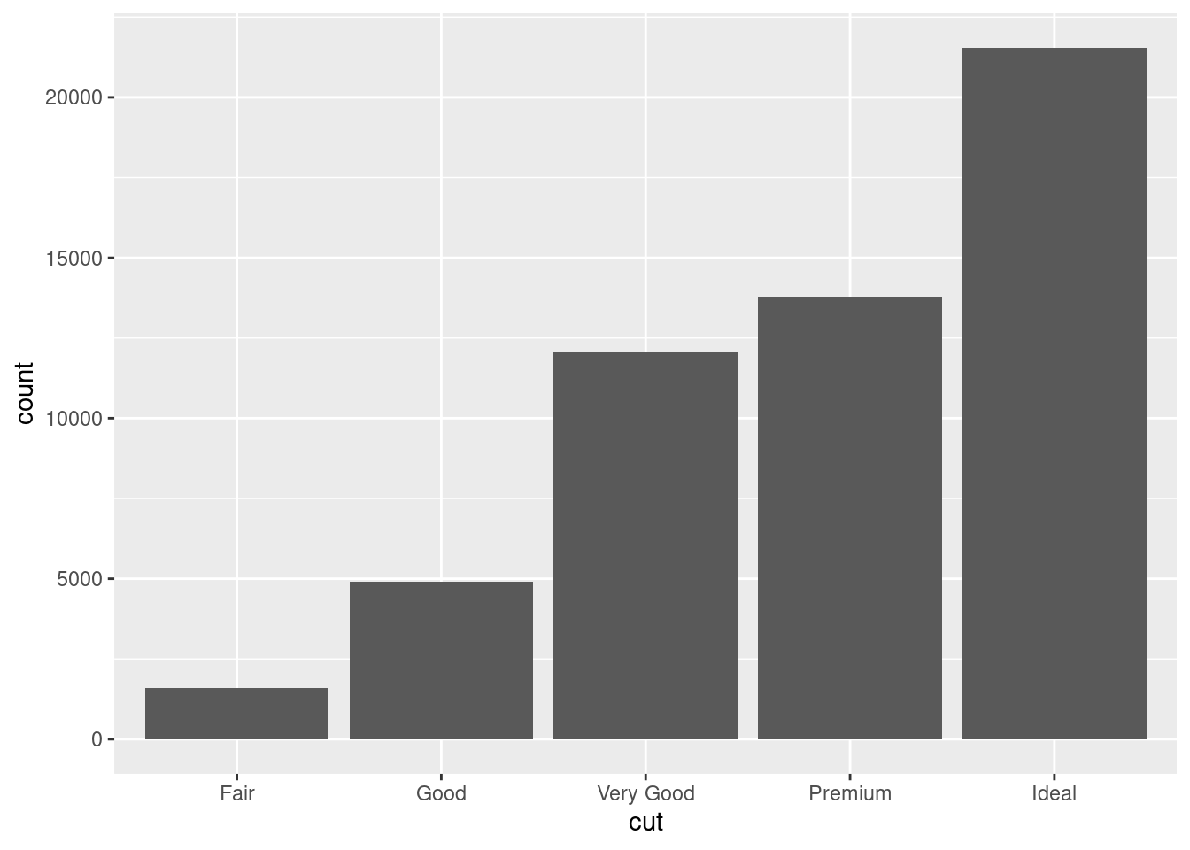
- categorical variable: can only take certain values. Visualize variation with bar chart.
ggplot(data = diamonds) +
  aes(x = cut) +
  geom_bar()
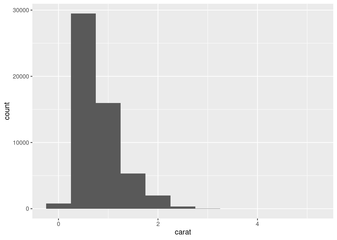
- continuous variables: can take on infinite set of ordered values. Visualize variation with histogram.
ggplot(data = diamonds) +
  aes(x = carat) +
  geom_histogram(binwidth = 0.5)
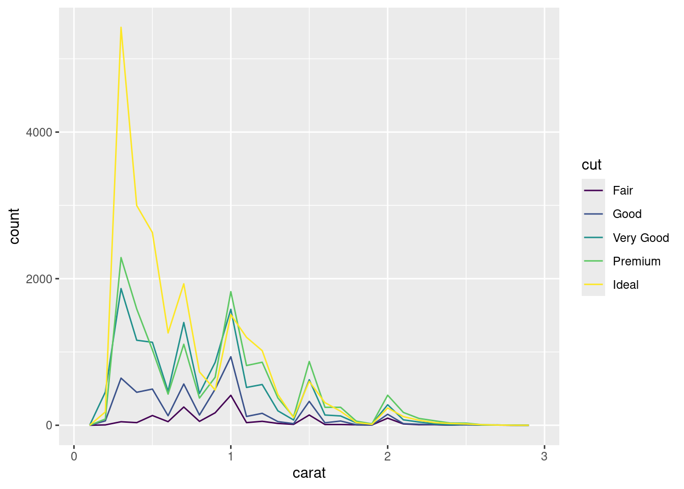
geom_freqpoly is geom_histogram alternative that doesn’t show bars.- Reminder: the
%>% pipe = “and then”.
{ggplot2} uses + to add layers, read it as “with” or “and”.
smaller <- diamonds %>%
  filter(carat < 3)
ggplot(smaller) +
  aes(x = carat, colour = cut) +
  geom_freqpoly(binwidth = 0.1)
- Use the visualizations to develop questions!
- Which values are the most common? Why?
- Which values are rare? Why? Does that match your expectations?
- Can you see any unusual patterns? What might explain them?
ggplot(smaller, mapping = aes(x = carat)) +
  geom_histogram(binwidth = 0.01)
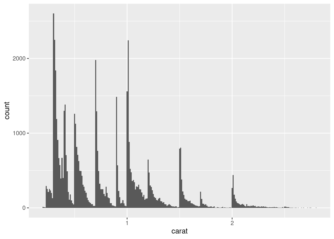
- Subgroups create more questions:
- How are the observations within each cluster similar to each other?
- How are the observations in separate clusters different from each other?
- How can you explain or describe the clusters?
- Why might the appearance of clusters be misleading?
- Use
coord_cartesian to zoom in to see unusual values.
- Can be ok to drop weird values, especially if you can explain where they came from.
- Always disclose that you did that, though.