18.4 Factors and empty groups

18.4.1 Factors and empty groups

A final type of missingness is the empty group, a group that doesn’t contain any observations, which can arise when working with factors.

Here is a dataset that contains some health information about people.

health <- tibble::tibble(
  name   = c("Ikaia", "Oletta", "Leriah", "Dashay", "Tresaun"),
  smoker = factor(c("no", "no", "no", "no", "no"), 
                  levels = c("yes", "no")),
  age    = c(34, 88, 75, 47, 56),
)

We want to count the number of smokers and non-smokers with dplyr::count() but it only gives us the amount of smokers because the group of smokers is empty

health |> dplyr::count(smoker)

## # A tibble: 1 × 2
##   smoker     n
##   <fct>  <int>
## 1 no         5

We can request count() to keep all the groups, even those not seen in the data by using .drop = FALSE:

health |> dplyr::count(smoker,
                       .drop = FALSE)

## # A tibble: 2 × 2
##   smoker     n
##   <fct>  <int>
## 1 yes        0
## 2 no         5

The same principle applies to ggplot2’s discrete axes, which will also drop levels that don’t have any values. You can force them to display by supplying drop = FALSE to the appropriate discrete axis

ggplot2::ggplot(
  data = health, 
  mapping = ggplot2::aes(
    x = .data[["smoker"]])
  ) +
  ggplot2::geom_bar() +
  ggplot2::scale_x_discrete()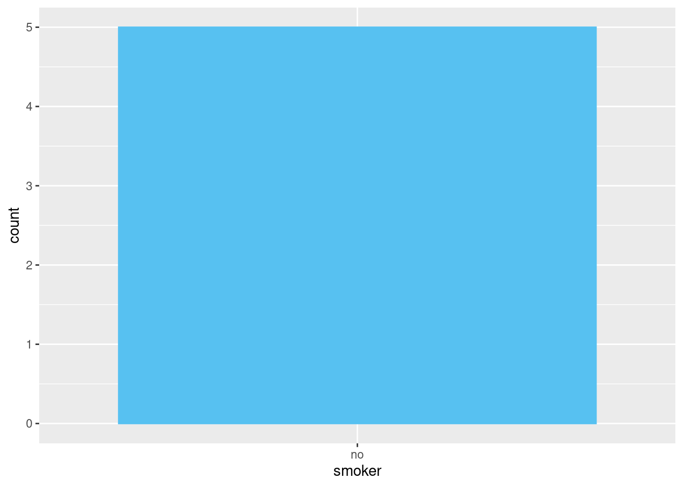

ggplot2::ggplot(
  data = health, 
  mapping = ggplot2::aes(
    x = .data[["smoker"]])
  ) +
  ggplot2::geom_bar() +
  ggplot2::scale_x_discrete(drop = FALSE)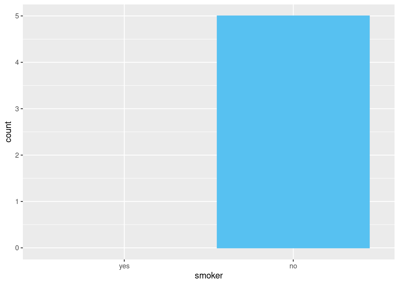

The same problem comes up more generally with dplyr::group_by(). And again you can use .drop = FALSE to preserve all factor levels:

health |> 
  dplyr::group_by(
    .data[["smoker"]]
  ) |> 
  dplyr::summarize(
    n = dplyr::n(),
    mean_age = mean(.data[["age"]]),
    min_age = min(.data[["age"]]),
    max_age = max(.data[["age"]]),
    sd_age = sd(.data[["age"]])
  )

## # A tibble: 1 × 6
##   smoker     n mean_age min_age max_age sd_age
##   <fct>  <int>    <dbl>   <dbl>   <dbl>  <dbl>
## 1 no         5       60      34      88   21.6

health |> 
  dplyr::group_by(
    .data[["smoker"]], 
    .drop = FALSE) |> 
  dplyr::summarize(
    n = dplyr::n(),
    mean_age = mean(.data[["age"]]),
    min_age = min(.data[["age"]]),
    max_age = max(.data[["age"]]),
    sd_age = sd(.data[["age"]])
  )

## Warning: There were 2 warnings in `dplyr::summarize()`.
## The first warning was:
## ℹ In argument: `min_age = min(.data[["age"]])`.
## ℹ In group 1: `smoker = yes`.
## Caused by warning in `min()`:
## ! no non-missing arguments to min; returning Inf
## ℹ Run `dplyr::last_dplyr_warnings()` to see the 1 remaining warning.

## # A tibble: 2 × 6
##   smoker     n mean_age min_age max_age sd_age
##   <fct>  <int>    <dbl>   <dbl>   <dbl>  <dbl>
## 1 yes        0      NaN     Inf    -Inf   NA  
## 2 no         5       60      34      88   21.6

We get some interesting results here because when summarizing an empty group, the summary functions are applied to zero-length vectors

Here we see mean({zero_vec}) returning NaN because

mean({zero_vec}) = sum({zero_vec})/length({zero_vec})

which is 0/0.

max() and min() return -Inf and Inf for empty vectors.

health |> 
  dplyr::group_by(
    .data[["smoker"]], 
    .drop = FALSE) |> 
  dplyr::summarize(
    n = dplyr::n(),
    mean_age = mean(.data[["age"]]),
    min_age = min(.data[["age"]]),
    max_age = max(.data[["age"]]),
    sd_age = sd(.data[["age"]])
  )

## Warning: There were 2 warnings in `dplyr::summarize()`.
## The first warning was:
## ℹ In argument: `min_age = min(.data[["age"]])`.
## ℹ In group 1: `smoker = yes`.
## Caused by warning in `min()`:
## ! no non-missing arguments to min; returning Inf
## ℹ Run `dplyr::last_dplyr_warnings()` to see the 1 remaining warning.

## # A tibble: 2 × 6
##   smoker     n mean_age min_age max_age sd_age
##   <fct>  <int>    <dbl>   <dbl>   <dbl>  <dbl>
## 1 yes        0      NaN     Inf    -Inf   NA  
## 2 no         5       60      34      88   21.6

Instead of .drop = FALSE, we can use tidyr::complete() to the implicit missing values explicit. The main drawback of this approach is that you get an NA for the count, even though you know that it should be zero.

health |> 
  dplyr::group_by(
    .data[["smoker"]]
  ) |> 
  dplyr::summarize(
    n = dplyr::n(),
    mean_age = mean(.data[["age"]]),
    min_age = min(.data[["age"]]),
    max_age = max(.data[["age"]]),
    sd_age = sd(.data[["age"]])
  ) |> 
  tidyr::complete(.data[["smoker"]])

## # A tibble: 2 × 6
##   smoker     n mean_age min_age max_age sd_age
##   <fct>  <int>    <dbl>   <dbl>   <dbl>  <dbl>
## 1 yes       NA       NA      NA      NA   NA  
## 2 no         5       60      34      88   21.6

18.4.2 forcats 1.0.0 Extra

Adapted from forcats 1.0.0 blog

There are two ways to represent a missing value in a factor:

NA as values:

f1 <- factor(c("x", "y", NA, NA, "x"), 
             exclude = NA)

levels(f1)

## [1] "x" "y"

NA as factors:

f2 <- factor(c("x", "y", NA, NA, "x"), 
             exclude = NULL)

levels(f2)

## [1] "x" "y" NA

They provide different behaviour when is.na and as.integer are applied

NA as values:

NAs in the values tend to be best for data analysis.

f1 <- factor(c("x", "y", NA, NA, "x"), 
             exclude = NA)

is.na(f1)

## [1] FALSE FALSE  TRUE  TRUE FALSE

as.integer(f1)

## [1]  1  2 NA NA  1

NA as factors:

NAs in the levels are useful if you need to control where missing values are shown in a table or a plot

f2 <- factor(c("x", "y", NA, NA, "x"), 
             exclude = NULL)

is.na(f2)

## [1] FALSE FALSE FALSE FALSE FALSE

as.integer(f2)

## [1] 1 2 3 3 1

To make it easier to switch between these forms, forcats now comes fct_na_value_to_level() and fct_na_level_to_value().

In the plot below, we use fct_infreq() to reorder the levels of the factor so that the highest frequency levels are at the top of the bar chart. However, because the NAs are stored in the values, fct_infreq() has no ability to affect them, so they appear in their “default” position.

example <- data.frame(
  hair_color = c(dplyr::starwars$hair_color, 
                 rep("missing", 10), 
                 rep("don't know", 5))
 ) |> 
  dplyr::mutate(
    hair_color = .data[["hair_color"]] |> 
      # Reorder factor by frequency
      forcats::fct_infreq() |> 
      # Group hair colours with less than 2 observations as Other
      forcats::fct_lump_min(2, other_level = "(Other)") |>
      forcats::fct_rev()
  ) 

example |> 
  ggplot2::ggplot(
    mapping = ggplot2::aes(
      y = .data[["hair_color"]]
    )
  ) + 
  ggplot2::geom_bar() + 
  ggplot2::labs(y = "Hair color")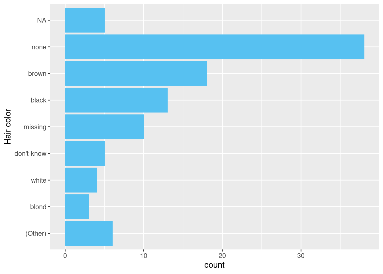

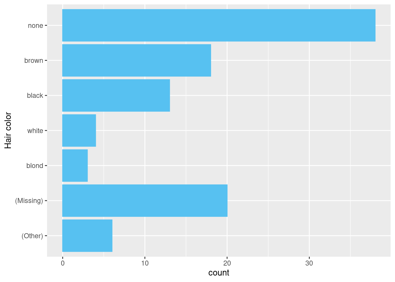
To consolidate all missing values,

• Use fct_recode to convert “don’t know” to the value “missing”.

• Use fct_na_level_to_value() to convert NA as a factor called “missing”.

• Use fct_na_value_to_level() to convert NA to the value “missing”.

example <- data.frame(
  hair_color = c(dplyr::starwars$hair_color, 
                 rep("missing", 10), 
                 rep("don't know", 5))
 ) |> 
  dplyr::mutate(
    hair_color = .data[["hair_color"]] |> 
      # Reorder factor by frequency
      forcats::fct_infreq() |> 
      forcats::fct_recode(
        missing = "don't know") |> 
      forcats::fct_na_level_to_value(
        extra_levels = "missing") |>
      forcats::fct_na_value_to_level(
        level = "(Missing)") |>
      # Group hair colours with less than 2 observations as Other
      forcats::fct_lump_min(2, other_level = "(Other)") |>
      forcats::fct_rev()
  )

example |> 
  ggplot2::ggplot(
    mapping = ggplot2::aes(
      y = .data[["hair_color"]]
    )
  ) + 
  ggplot2::geom_bar() + 
  ggplot2::labs(y = "Hair color")