5.3 Weighted Data

If each row of your dataframe contains multiple observations, we can use a weight to visually give scale to observations

# Unweighted
ggplot(midwest, aes(percwhite, percbelowpoverty)) + 
  geom_point()

# Weight by population
ggplot(midwest, aes(percwhite, percbelowpoverty)) + 
  geom_point(aes(size = poptotal / 1e6)) + 
  scale_size_area("Population\n(millions)", breaks = c(0.5, 1, 2, 4))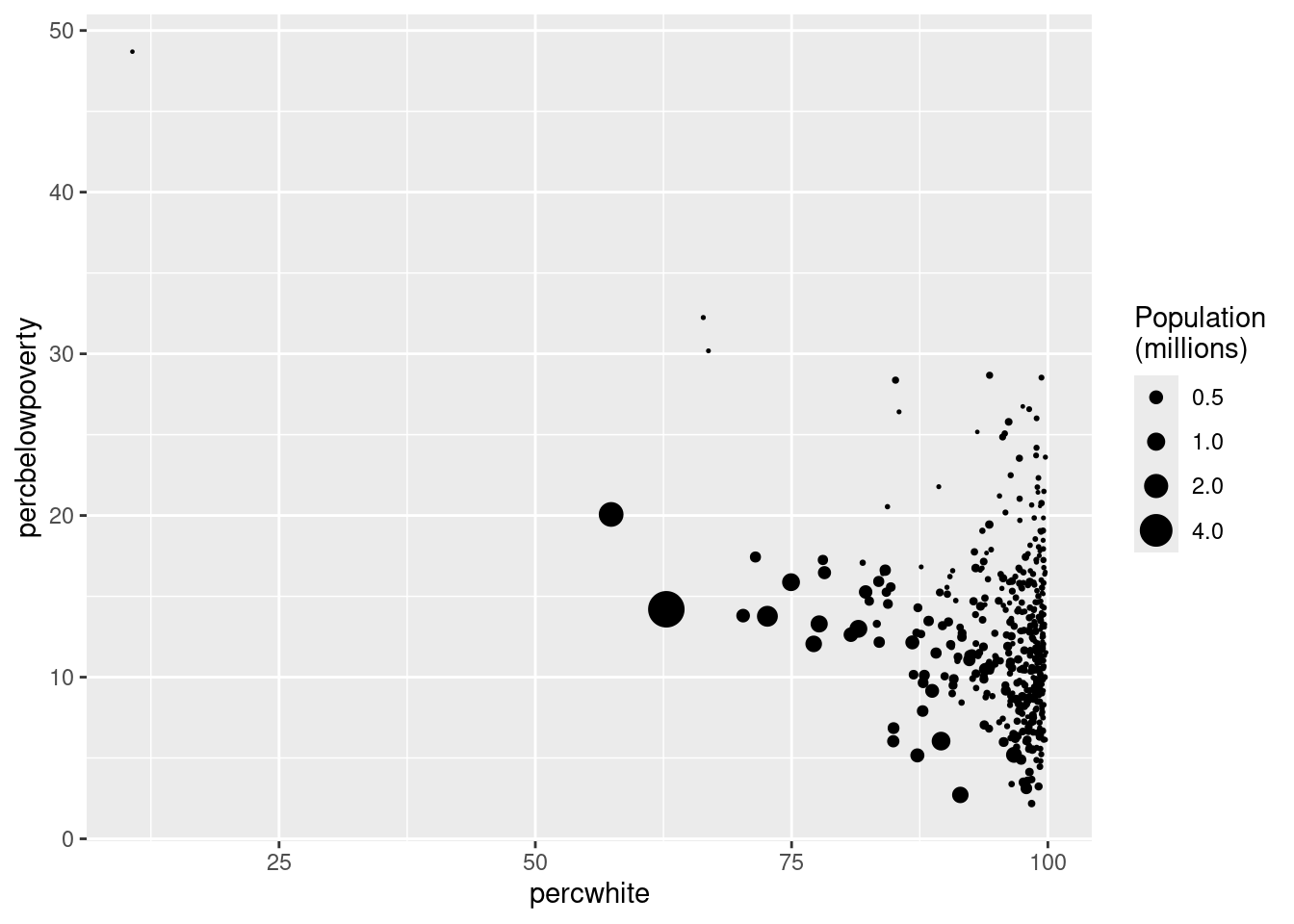

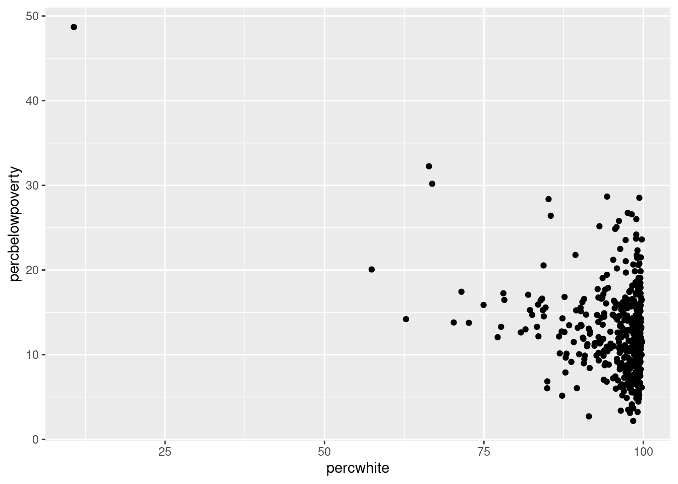
# Unweighted
ggplot(midwest, aes(percwhite, percbelowpoverty)) + 
  geom_point() + 
  geom_smooth(method = lm, size = 1)

## `geom_smooth()` using formula = 'y ~ x'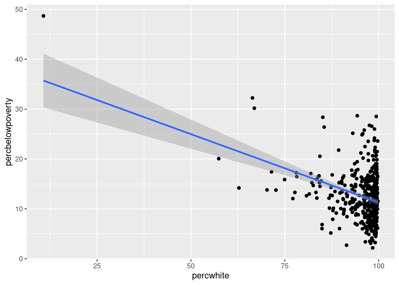

# Weighted by population
ggplot(midwest, aes(percwhite, percbelowpoverty)) + 
  geom_point(aes(size = poptotal / 1e6)) + 
  geom_smooth(aes(weight = poptotal), method = lm, size = 1) +
  scale_size_area(guide = "none")

## `geom_smooth()` using formula = 'y ~ x'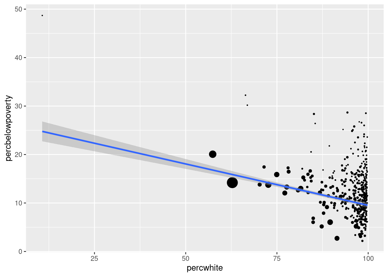

ggplot(midwest, aes(percbelowpoverty)) +
  geom_histogram(binwidth = 1) + 
  ylab("Counties")

ggplot(midwest, aes(percbelowpoverty)) +
  geom_histogram(aes(weight = poptotal), binwidth = 1) +
  ylab("Population (1000s)")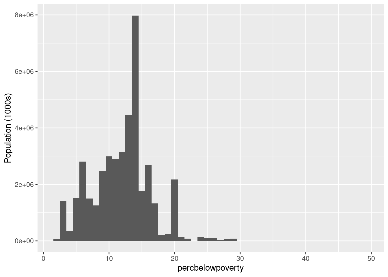

Question for the group: Is the above ylab correct? Check out the next two figures, can you see the difference?

ggplot(midwest, aes(percbelowpoverty)) +
  geom_histogram(aes(weight = poptotal/1e3), binwidth = 1) +
  ylab("Population (1000s)")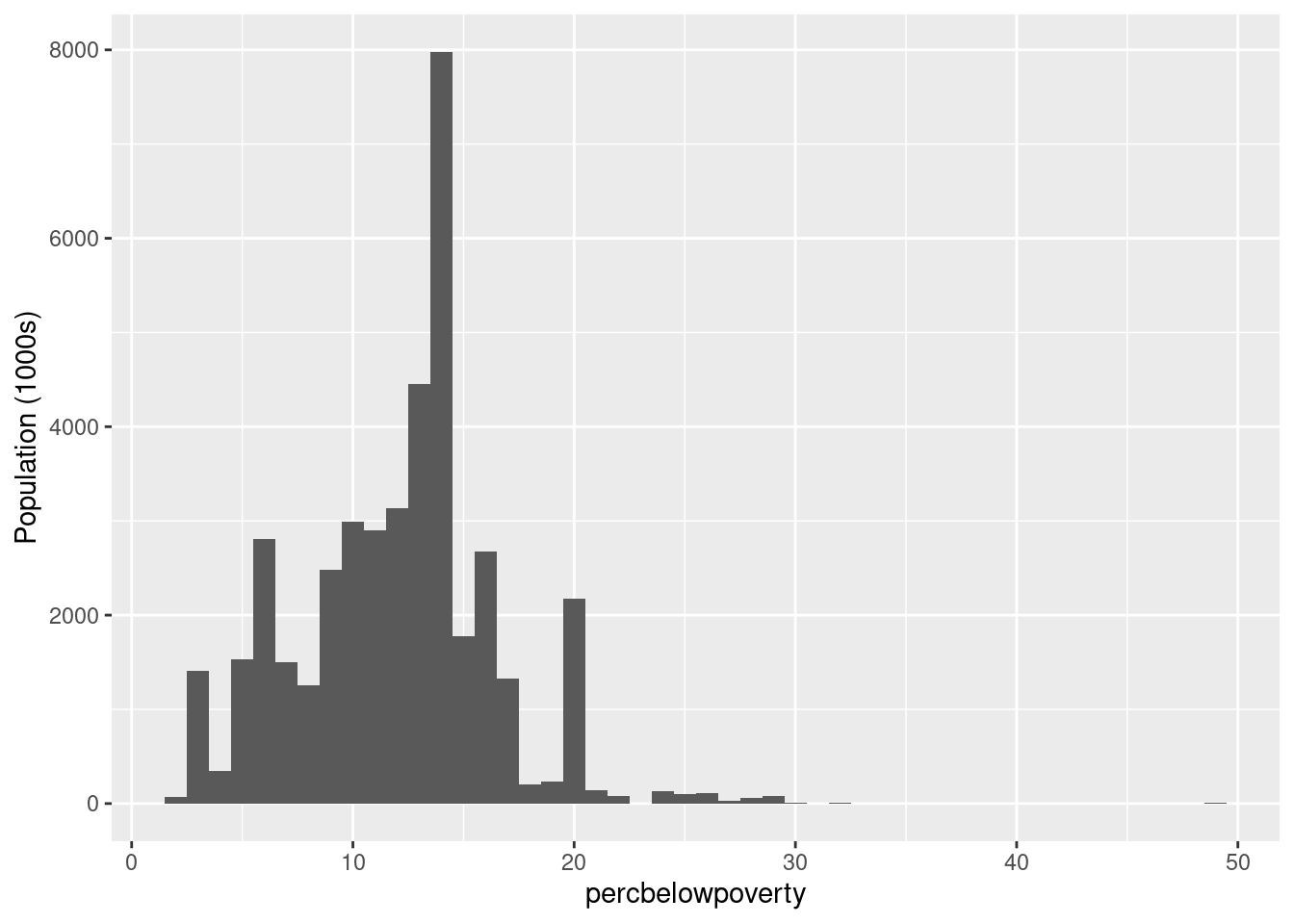

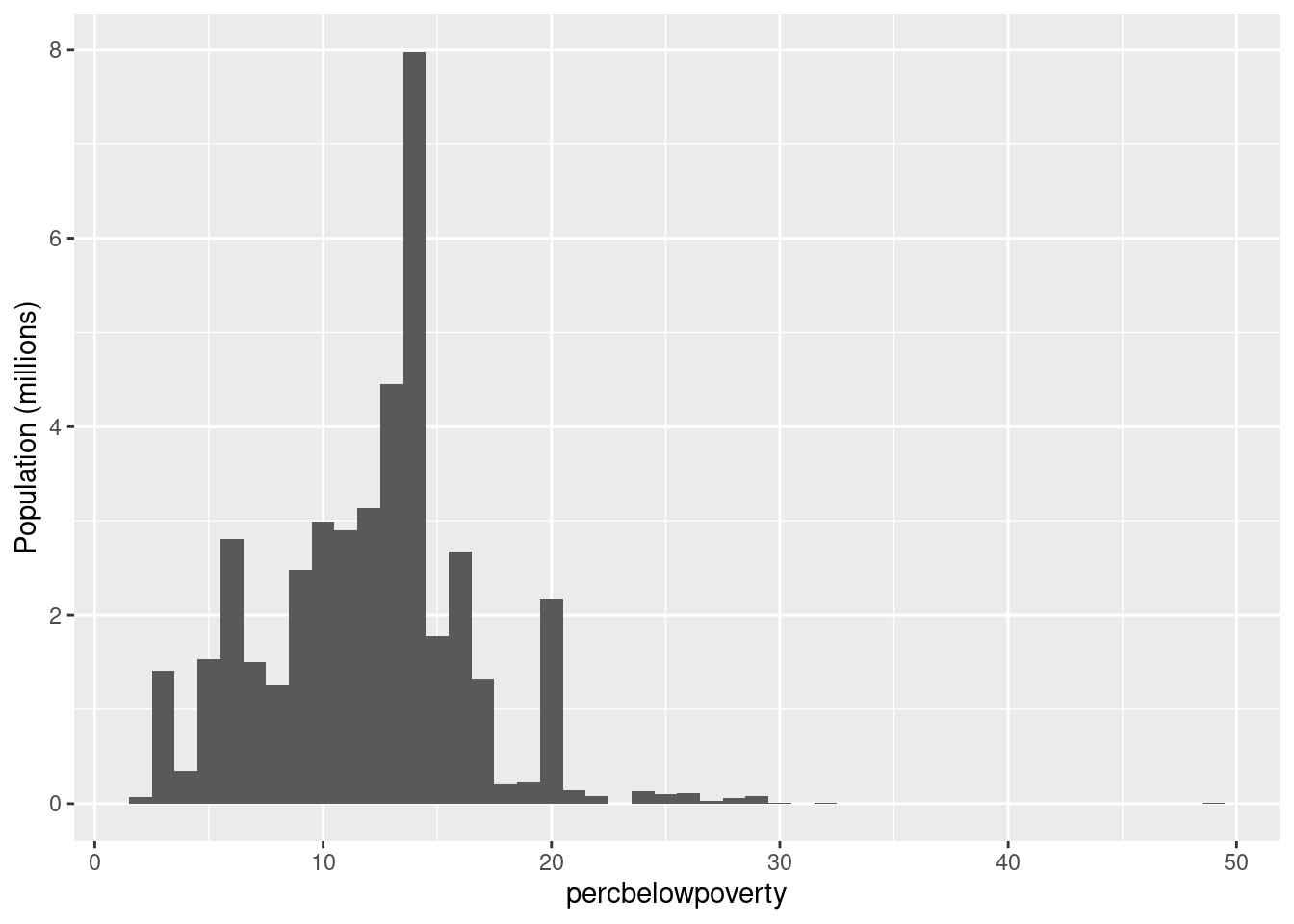
ggplot(midwest, aes(percbelowpoverty)) +
  geom_histogram(aes(weight = poptotal/1e6), binwidth = 1) +
  ylab("Population (millions)")