13.1 Building a plot
In this chapter we talk about the grammar of graphics plots and their construction layer by layer.
We use data from the {SpatialEpi} package:
Let’s check what data is inside the package, we can use the NYleukemia which contains observations about leukemia cases in NY, as well as providing other information about population and spatials such as latidude and logitude where the cases were located.
##   censustract.FIPS   cases population
## 1      36007000100 3.08284       3540
## 2      36007000200 4.08331       3560
## 3      36007000300 1.08750       3739
## censustract.FIPS x y
## 1 36007000100 -75.94087 42.10782
## 2 36007000200 -75.93118 42.11099
## 3 36007000300 -75.92011 42.11738Let’s now make a first layer visualization using ggplot2

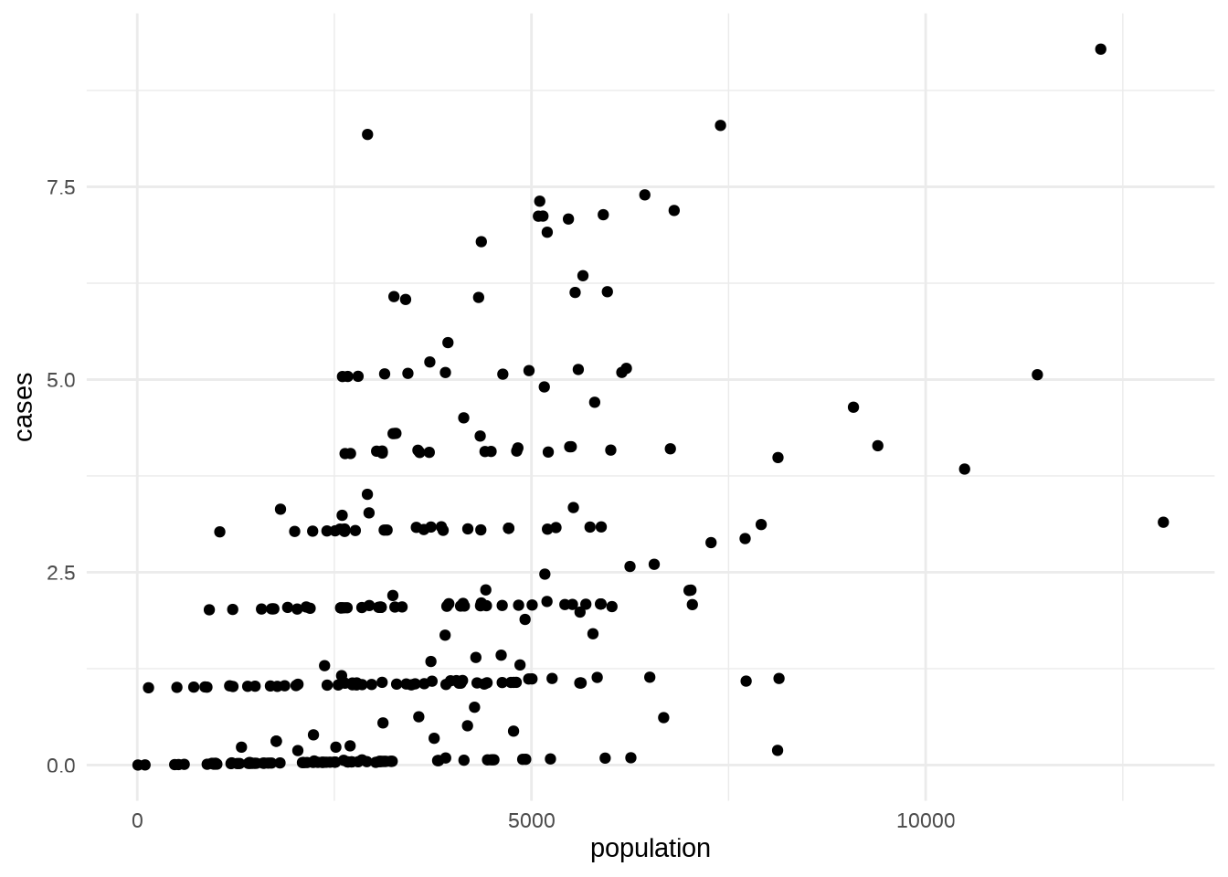
The second layer of our plot would take consideration of the geoms

In general when we make a ggplot, we build the plot without thinking about the layers, but what is happening inside the hood when we add a layer?
The layer() function is called for combining data, stat and geom.
Layers are created using geom_* or stat_* calls or directly using the function:
  layer(
    geom = NULL,
    stat = NULL,
    data = NULL,
    mapping = NULL,
    position = NULL,
    params = list(),
    inherit.aes = TRUE,
    check.aes = TRUE,
    check.param = TRUE,
    show.legend = NA,
    key_glyph = NULL,
    layer_class = Layer
  )
To obtain the same results:
layer() function components:
- mapping
- data
- geom
- stat
- position
- …