19.1 The plot() method

The user-facing code and internal code is also separated by when they are evaluated. The user-facing code like geom_smooth() is evaluated immediately to give you a ggplot object, but the internal code is only evaluated when a ggplot object is printed or plotted, via print() and plot().

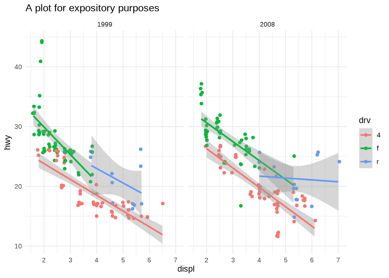
The following code simply creates a ggplot object from user-facing code, and DOES NOT print or plot the ggplot (yet).

p <- ggplot(mpg, aes(displ, hwy, color = drv)) + 
  geom_point(position = position_jitter(seed = 2022)) +
  geom_smooth(method = "lm", formula = y ~ x) + 
  facet_wrap(vars(year)) + 
  ggtitle("A plot for expository purposes")

The ggplot object is actually just a list under the hood:

class(p)

[1] "gg"     "ggplot"

typeof(p)

[1] "list"

Evaluating the ggplot is what gives you the actual points, rectangles, text, etc. that make up the figure (and you can also do so explicitly with print()/plot())

p

# print(p)
# plot(p)

These are two separate processes, but we often think of them as one monolithic process:

defining_benchmark <- bench::mark(
  # Evaluates user-facing code to define ggplot,
  # but does not call plot/print method
  p <- ggplot(mpg, aes(displ, hwy, color = drv)) + 
    geom_point(position = position_jitter(seed = 2022)) +
    geom_smooth(method = "lm", formula = y ~ x) + 
    facet_wrap(vars(year)) + 
    ggtitle("A plot for expository purposes")
)

plotting_benchmark <- bench::mark(
  # Plots the ggplot
  plot(p)
)

bind_rows(
  defining_benchmark[,2:5],
  plotting_benchmark[,2:5]
)

# A tibble: 2 × 4
       min   median `itr/sec` mem_alloc
  <bch:tm> <bch:tm>     <dbl> <bch:byt>
1   3.15ms   3.25ms    299.     30.34KB
2 238.85ms 239.43ms      4.18    3.58MB

The plot that gets rendered from a ggplot object is actually a side effect of evaluating the ggplot object:

# Same as ggplot2:::print.ggplot
ggplot2:::plot.ggplot

function (x, newpage = is.null(vp), vp = NULL, ...) 
{
    set_last_plot(x)
    if (newpage) 
        grid.newpage()
    grDevices::recordGraphics(requireNamespace("ggplot2", quietly = TRUE), 
        list(), getNamespace("ggplot2"))
    data <- ggplot_build(x)
    gtable <- ggplot_gtable(data)
    if (is.null(vp)) {
        grid.draw(gtable)
    }
    else {
        if (is.character(vp)) 
            seekViewport(vp)
        else pushViewport(vp)
        grid.draw(gtable)
        upViewport()
    }
    if (isTRUE(getOption("BrailleR.VI")) && rlang::is_installed("BrailleR")) {
        print(asNamespace("BrailleR")$VI(x))
    }
    invisible(x)
}
<bytecode: 0x5626733081f8>
<environment: namespace:ggplot2>

The above code can be simplified to this:

ggprint <- function(x) {
  data <- ggplot_build(x)
  gtable <- ggplot_gtable(data)
  grid::grid.newpage()
  grid::grid.draw(gtable)
  return(invisible(x)) #< hence "side effect"
}

ggprint(p)

Roughly put, you first start out as the ggplot object, which then gets passed to ggplot_build(), result of which in turn gets passed to ggplot_gtable() and finally drawn with {grid}

library(grid)
grid.newpage() # Clear display
p %>% 
  ggplot_build() %>%  # 1. data for each layer is prepared for drawing
  ggplot_gtable() %>% # 2. drawing-ready data is turned into graphical elements
  grid.draw()         # 3. graphical elements are converted to an image

At each step, you get closer to the low-level information you need to draw the actual plot

obj_byte <- function(x) {
  scales::label_bytes()(as.numeric(object.size(x)))
}

# ggplot object
p %>% obj_byte()

[1] "32 kB"

# data used to make graphical elements
ggplot_build(p) %>% obj_byte()

[1] "102 kB"

# graphical elements for the plot
ggplot_gtable(ggplot_build(p)) %>% obj_byte()

[1] "685 kB"

# the rendered plot
ggsave(
  filename = tempfile(fileext = ".png"),
  plot = ggplot_gtable(ggplot_build(p)),
  # File size depends on format, dimension, resolution, etc.
) %>% file.size() %>% {scales::label_bytes()(.)}

[1] "243 kB"

The rest of the chapter focuses what happens in this pipeine - the ggplot_build() step and the ggplot_gtable() step.