13.2 Data
The layers of your plot can be populated with different datasets.
Here we generate two new datasets from the df dataset.
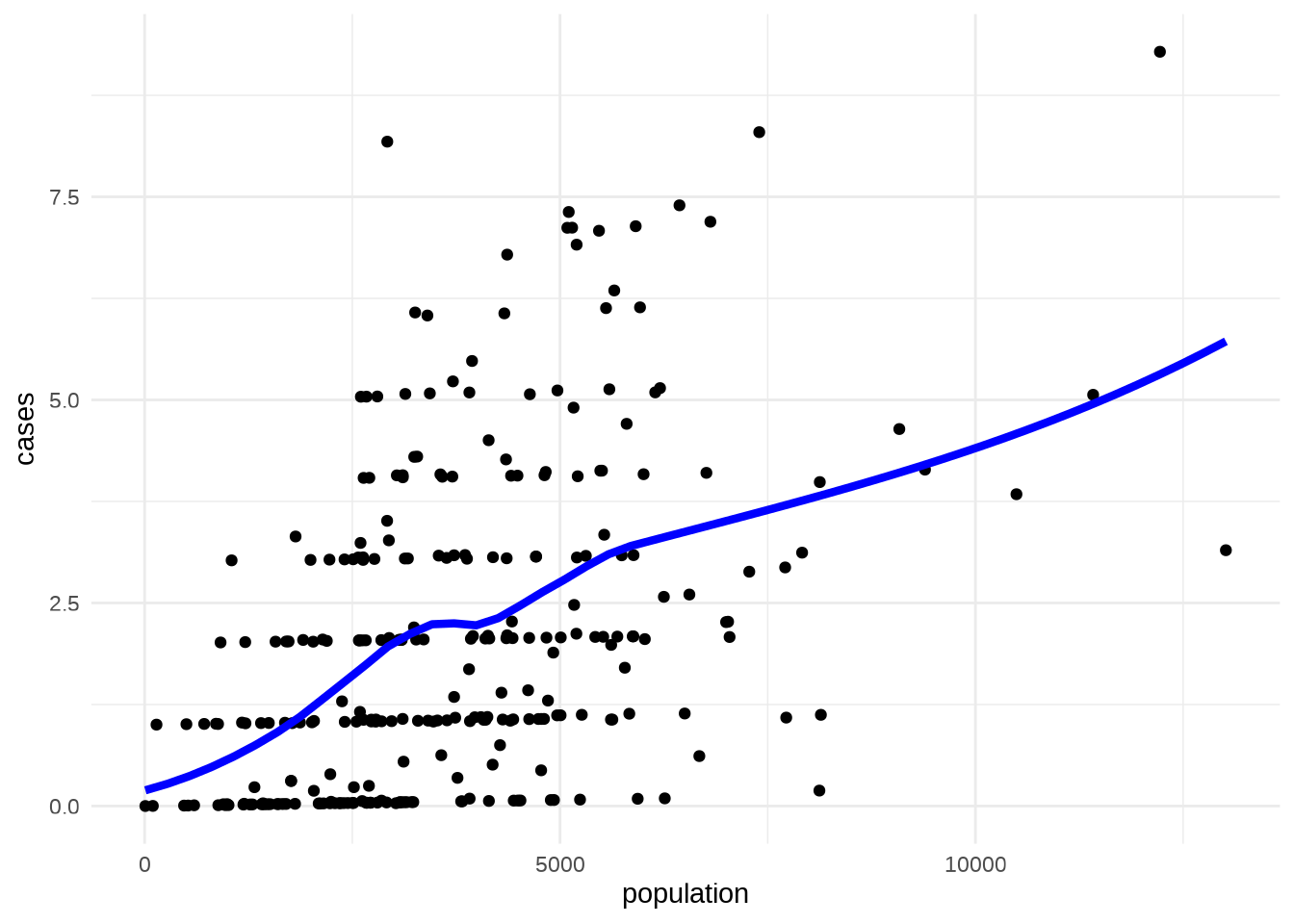
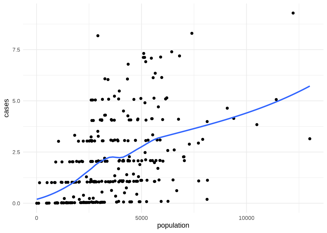
What geom_smooth() does behind the scenes?
- fit a model, in this case a loess model
- generate prediction, about the trend of the data
In this example we create a grid of length of 50 to have an average trend to show in a secondary layer of the plot.
## # A tibble: 3 × 2
##   population cases
##        <dbl> <dbl>
## 1         9  0.194
## 2       274. 0.273
## 3       540. 0.369
## [1] 50 2## [1] 281 5Next step would be to isolate the outliers (observations far away from predicted values), with the help of the resid() function to extract model residuals
## Call:
## loess(formula = cases ~ population, data = df)
##
## Number of Observations: 281
## Equivalent Number of Parameters: 5.33
## Residual Standard Error: 1.769
## Trace of smoother matrix: 5.84  (exact)
##
## Control settings:
##   span     :  0.75
##   degree   :  2
##   family   :  gaussian
##   surface  :  interpolate      cell = 0.2
##   normalize:  TRUE
##  parametric:  FALSE
## drop.square:  FALSE
And build the residuals std error vector:
##   censustract.FIPS   cases population         x        y
## 1      36007012500 7.13834       5911 -75.69563 42.06164
## 2      36007013000 7.11907       5088 -76.00001 42.12407
## 3      36007013302 0.19008       8122 -76.06948 42.13547
## [1] 16 5Add a new layer with different data: grid


