5.6 Statistical Summaries
geom_histogram() and geom_bin2d() use a familiar geom, geom_bar() and geom_raster(), combined with a new statistical transformation, stat_bin() and stat_bin2d(). stat_bin() and stat_bin2d() combine the data into bins and count the number of observations in each bin. But what if we want a summary other than count? So far, we’ve just used the default statistical transformation associated with each geom. Now we’re going to explore how to use stat_summary_bin() to stat_summary_2d() to compute different summaries.
-1.png)
-2.png)
ggplot(diamonds, aes(table, depth)) +
  geom_bin2d(binwidth = 1, na.rm = TRUE) +
  xlim(50, 70) +
ylim(50, 70)-1.png)
ggplot(diamonds, aes(table, depth, z = price)) +
  geom_raster(binwidth = 1, stat = "summary_2d", fun = mean,
    na.rm = TRUE) +
  xlim(50, 70) +
  ylim(50, 70)
## Warning: Raster pixels are placed at uneven horizontal intervals and will be shifted
## ℹ Consider using `geom_tile()` instead.
## Raster pixels are placed at uneven horizontal intervals and will be shifted
## ℹ Consider using `geom_tile()` instead.-2.png)
So far we’ve considered two classes of geoms:
Simple geoms where there’s a one-on-one correspondence between rows in the data frame and physical elements of the geom
Statistical geoms where introduce a layer of statistical summaries in between the raw data and the result
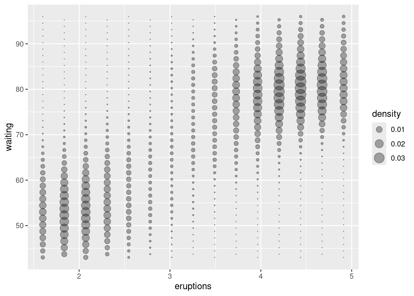
Although ggplot2 does not have direct 3d support, it does provide the ability to plot 2d images representing 3d data. These include: contours, colored tiles, and bubble plots.
## Warning: The dot-dot notation (`..level..`) was deprecated in ggplot2 3.4.0.
## ℹ Please use `after_stat(level)` instead.
## This warning is displayed once every 8 hours.
## Call `lifecycle::last_lifecycle_warnings()` to see where this warning was
## generated.-1.png)
-1.png)
# Bubble plots work better with fewer observations
small <- faithfuld[seq(1, nrow(faithfuld), by = 10), ]
ggplot(small, aes(eruptions, waiting)) +
  geom_point(aes(size = density), alpha = 1/3) +
  scale_size_area()