22.3 Scaling
“The values in the previous table have no meaning to the computer. We need to convert them from data units (e.g., litres, miles per gallon and number of cylinders) to graphical units (e.g., pixels and colours) that the computer can display. This conversion process is called scaling and performed by scales.”
what we see to what the computer reads
- we see colours; computer reads hexadecimal string
- we see size; computer reads a number
- we see shapes; the computer reads an integer
Example in Page 4-6 of Wickham, H. (2010)
“Scales typically map from a single variable to a single aesthetic, but there are exceptions. For example, we can map one variable to hue and another to saturation, to create a single aesthetic, color. We can also create redundant mappings, mapping the same variable to multiple aesthetics.” (Wickham, 2010, p. 13)
These aesthetic specifications that are meaningful to R are described in vignette(“ggplot2-specs”)
Shape Shapes take five types of values:
An integer in [0,25]:
shapes <- data.frame(
  shape = c(0:19, 22, 21, 24, 23, 20),
  x = 0:24 %/% 5,
  y = -(0:24 %% 5)
)
ggplot(shapes, aes(x, y)) +
  geom_point(aes(shape = shape), size = 5, fill = "red") +
  geom_text(aes(label = shape), hjust = 0, nudge_x = 0.15) +
  scale_shape_identity() +
  expand_limits(x = 4.1) +
  theme_void()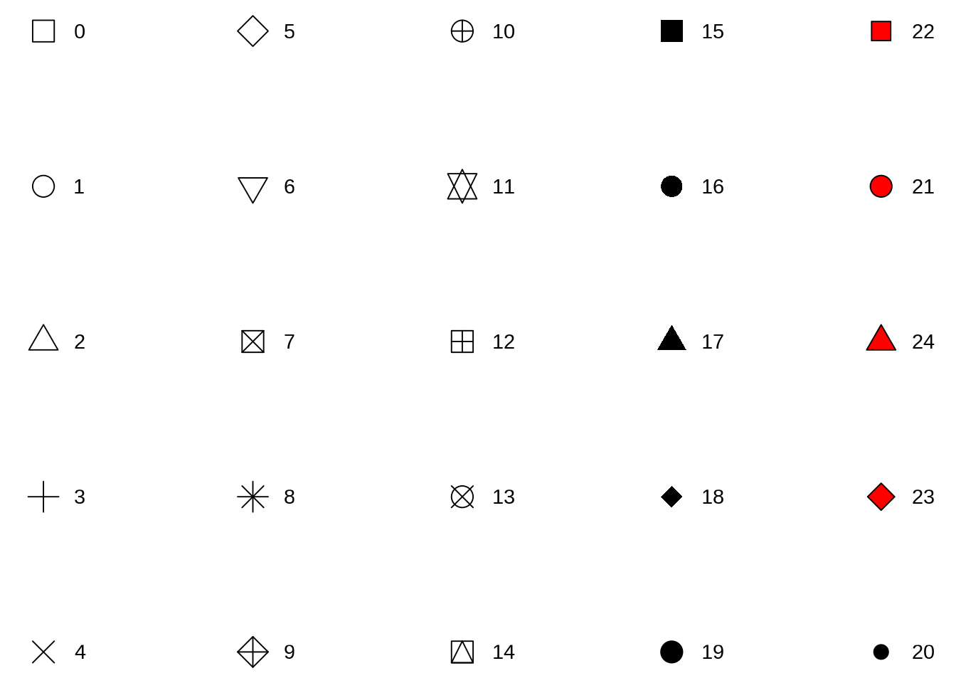
Line type Line types can be specified with:
An integer or name: 0 = blank, 1 = solid, 2 = dashed, 3 = dotted, 4 = dotdash, 5 = longdash, 6 = twodash, as shown below:
lty <- c("solid", "dashed", "dotted", "dotdash", "longdash", "twodash")
linetypes <- data.frame(
  y = seq_along(lty),
  lty = lty
)
ggplot(linetypes, aes(0, y)) +
  geom_segment(aes(xend = 5, yend = y, linetype = lty)) +
  scale_linetype_identity() +
  geom_text(aes(label = lty), hjust = 0, nudge_y = 0.2) +
  scale_x_continuous(NULL, breaks = NULL) +
  scale_y_reverse(NULL, breaks = NULL)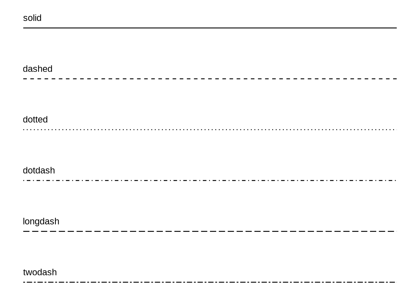
Font face There are only three fonts that are guaranteed to work everywhere: “sans” (the default), “serif”, or “mono”:
df <- data.frame(x = 1, y = 3:1, family = c("sans", "serif", "mono"))
ggplot(df, aes(x, y)) +
  geom_text(aes(label = family, family = family))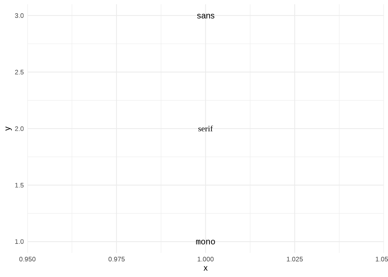
Colour and fill Note that shapes 21-24 have both stroke colour and a fill. The size of the filled part is controlled by size, the size of the stroke is controlled by stroke. Each is measured in mm, and the total size of the point is the sum of the two. Note that the size is constant along the diagonal in the following figure.
sizes <- expand.grid(size = (0:3) * 2, stroke = (0:3) * 2)
ggplot(sizes, aes(size, stroke, size = size, stroke = stroke)) +
  geom_abline(slope = -1, intercept = 6, colour = "white", size = 6) +
  geom_point(shape = 21, fill = "red") +
  scale_size_identity()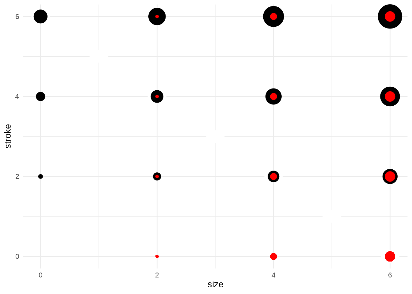
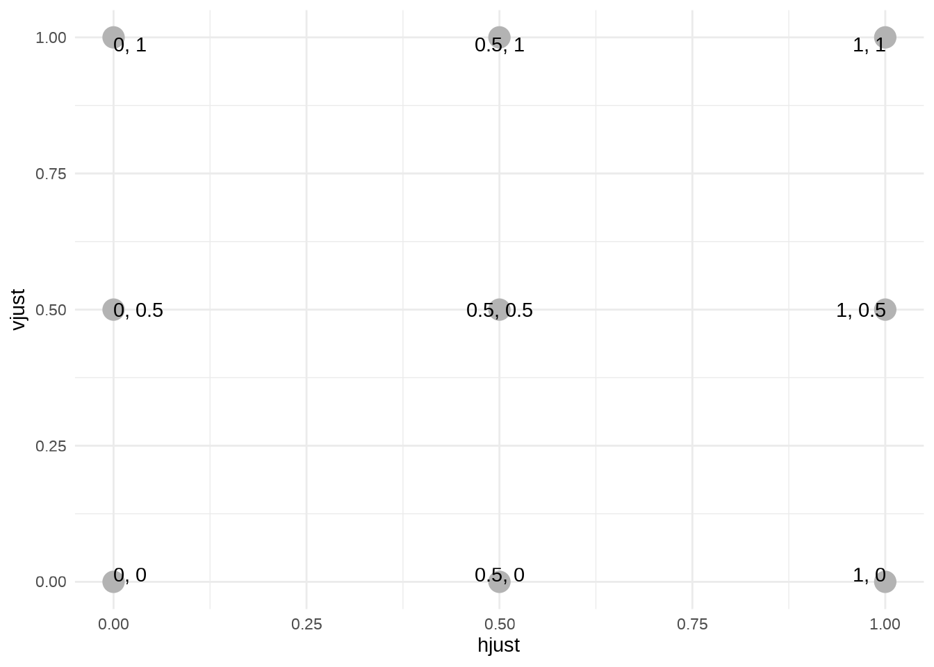
Horizontal and vertical justification have the same parameterisation, either a string (“top”, “middle”, “bottom”, “left”, “center”, “right”) or a number between 0 and 1:
top = 1, middle = 0.5, bottom = 0 left = 0, center = 0.5, right = 1
just <- expand.grid(hjust = c(0, 0.5, 1), vjust = c(0, 0.5, 1))
just$label <- paste0(just$hjust, ", ", just$vjust)

ggplot(just, aes(hjust, vjust)) +
  geom_point(colour = "grey70", size = 5) +
  geom_text(aes(label = label, hjust = hjust, vjust = vjust))