14.3 Scale Limits
Section 15.1 introduced the concept that a scale defines a mapping from the data space to the aesthetic space.
Scale limits are an extension of this idea: they dictate the region of the data space over which the mapping is defined.
For continuous and binned scales, the data space is inherently continuous and one-dimensional, so the limits can be specified by two end points.
For discrete scales, however, the data space is unstructured and consists only of a set of categories: as such the limits for a discrete scale can only be specified by enumerating the set of categories over which the mapping is defined.
The toolbox chapters outline the common practical goals for specifying the limits: for position scales the limits are used to set the end points of the axis, for example.
This leads naturally to the question of what ggplot2 should do if the data set contains “out of bounds” values that fall outside the limits.
The default behaviour in ggplot2 is to convert out of bounds values to NA.
We can override this default by setting
oobargument of the scale, a function that is applied to all observations outside the scale limits.The default is
scales::oob_censor()which replaces any value outside the limits withNA.Another option is
scales::oob_squish()which squishes all values into the range. An example using a fill scale is shown below:


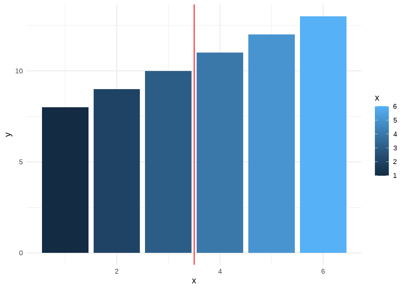
The first plot the default fill colours are shown, ranging from dark blue to light blue.
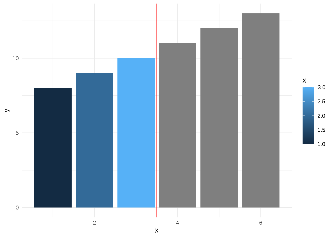
In the second plot the scale limits for the fill aesthetic are reduced so that the values for the three rightmost bars are replace with NA and are mapped to a grey shade.
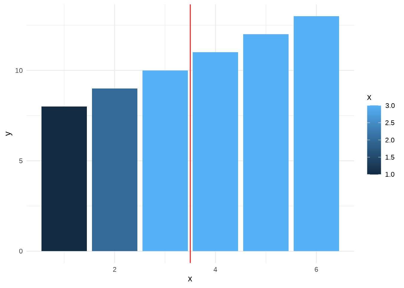
In some cases this is desired behaviour but often it is not: the third plot addresses this by modifying the oob function appropriately.