19.5 Steps

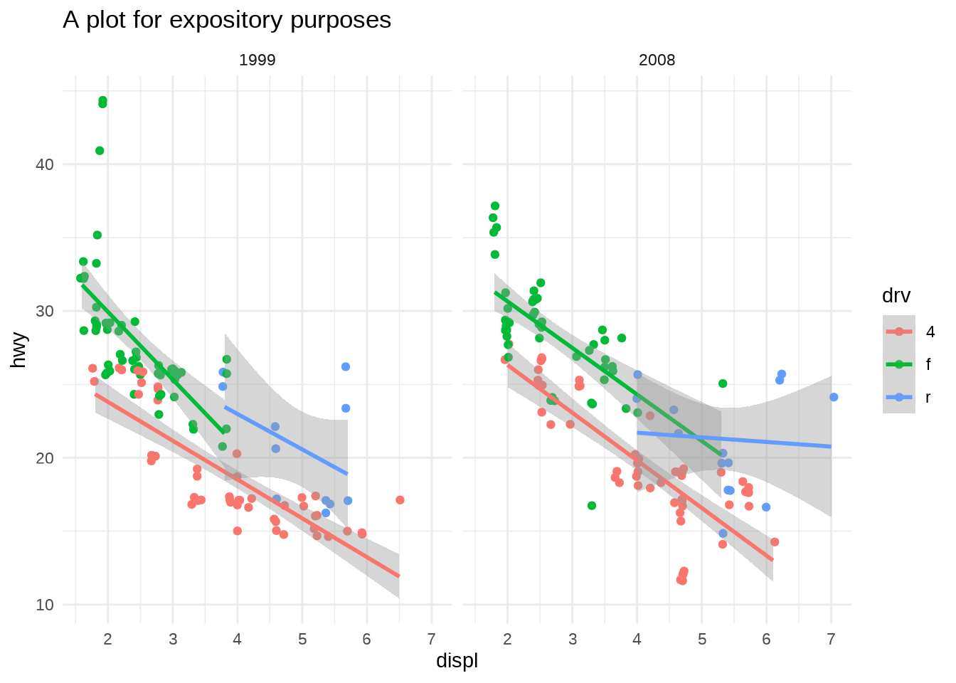
The plot that gets rendered from a ggplot object is actually a side effect of evaluating the ggplot object:

ggplot object

# Same as ggplot2:::print.ggplot
ggplot2:::plot.ggplot

function (x, newpage = is.null(vp), vp = NULL, ...) 
{
    set_last_plot(x)
    if (newpage) 
        grid.newpage()
    grDevices::recordGraphics(requireNamespace("ggplot2", quietly = TRUE), 
        list(), getNamespace("ggplot2"))
    data <- ggplot_build(x)
    gtable <- ggplot_gtable(data)
    if (is.null(vp)) {
        grid.draw(gtable)
    }
    else {
        if (is.character(vp)) 
            seekViewport(vp)
        else pushViewport(vp)
        grid.draw(gtable)
        upViewport()
    }
    if (isTRUE(getOption("BrailleR.VI")) && rlang::is_installed("BrailleR")) {
        print(asNamespace("BrailleR")$VI(x))
    }
    invisible(x)
}
<bytecode: 0x55a50675de40>
<environment: namespace:ggplot2>

The above code can be simplified to this:

ggprint <- function(x) {
  data <- ggplot_build(x)
  gtable <- ggplot_gtable(data)
  grid::grid.newpage()
  grid::grid.draw(gtable)
  return(invisible(x)) #< hence "side effect"
}

ggprint(p)

Roughly put, you first start out as the ggplot object, which then gets passed to ggplot_build(), result of which in turn gets passed to ggplot_gtable() and finally drawn with {grid}

library(grid)
grid.newpage() # Clear display
p %>% 
  ggplot_build() %>%  # 1. data for each layer is prepared for drawing
  ggplot_gtable() %>% # 2. drawing-ready data is turned into graphical elements
  grid.draw()         # 3. graphical elements are converted to an image

At each step, you get closer to the low-level information you need to draw the actual plot

# ggplot object
p %>% obj_byte()

[1] "32 kB"

# data used to make graphical elements
ggplot_build(p) %>% obj_byte()

[1] "102 kB"

# graphical elements for the plot
ggplot_gtable(ggplot_build(p)) %>% obj_byte()

[1] "685 kB"

# the rendered plot
ggsave(
  filename = tempfile(fileext = ".png"),
  plot = ggplot_gtable(ggplot_build(p)),
  # File size depends on format, dimension, resolution, etc.
) %>% file.size() %>% {scales::label_bytes()(.)}

[1] "243 kB"

The rest of the chapter focuses what happens in this pipeline - the ggplot_build() step and the ggplot_gtable() step.