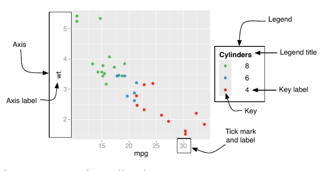
14.1 Theory of scales and guides
Each scale is a function from a region in data space to a region in aesthetic space.
The axis or legend is the inverse function, known as the guide: it allows you to convert visual properties back to data.
Surprisingly, axes and legends are the same type of thing, but while they look very different they have the same purpose: to allow you to read observations from the plot and map them back to their original values.
The commonalities between the two are illustrated below:
| Argument name | Axis | Legend |
|---|---|---|
name |
Label | Title |
breaks |
Ticks & grid line | Key |
labels |
Tick label | Key label |

However, legends are more complicated than axes, and consequently there are a number of topics that are specific to legends:
1. A legend can display multiple aesthetics (e.g. colour and shape), from multiple layers (Section 15.7.1), and the symbol displayed in a legend varies based on the geom used in the layer (Section 15.8)
2. Axes always appear in the same place. Legends can appear in different places, so you need some global way of positioning them. (Section 11.7)
3. Legends have more details that can be tweaked: should they be displayed vertically or horizontally? How many columns? How big should the keys be? This is discussed in (Section 15.5)
14.1.1 Scale specification
An important property of ggplot2 is the principle that every aesthetic in your plot is associated with exactly one scale. For instance, when you write this
ggplot2 adds a default scale for each aesthetic used in the plot:
ggplot(mpg, aes(displ, hwy)) +
geom_point(aes(colour = class)) +
scale_x_continuous() +
scale_y_continuous() +
scale_colour_discrete()ggplot(mpg, aes(displ, hwy)) +
geom_point(aes(colour = class)) +
scale_x_continuous(name = "A really awesome x axis label") +
scale_y_continuous(name = "An amazingly great y axis label")The use of + to “add” scales to a plot is a little misleading because if you supply two scales for the same aesthetic, the last scale takes precedence:
ggplot(mpg, aes(displ, hwy)) +
  geom_point() +
  scale_x_continuous(name = "Label 1") +
  scale_x_continuous(name = "Label 2")
#> Scale for 'x' is already present. Adding another scale for 'x', which will
#> replace the existing scale.

ggplot(mpg, aes(displ, hwy)) +
  geom_point() +
scale_x_continuous(name = "Label 2")14.1.2 Naming scheme
The scale functions intended for users all follow a common naming scheme. You’ve probably already figured out the scheme, but to be concrete, it’s made up of three pieces separated by “_“:
1. scale
2. The name of the primary aesthetic (e.g., colour, shape or x)
3. The name of the scale (e.g., continuous, discrete, brewer).
14.1.3 Fundamental scale types
All scale functions in ggplot2 belong to one of three fundamental types:
- continuous scales,
- discrete scales, and
- binned scales.
Each fundamental type is handled by one of three scale constructor functions:
continuous_scale(),discrete_scale()andbinned_scale().
Although you should never need to call these constructor functions, they provide the organizing structure for scales and it is useful to know about them.