3.1 Vector Objects
The sf package builds on the data.frame, adding a sticky sfc class column that contain wide a range of geographic entities.

This is a huge package, with more than one hundred methods, including
aggregate, rbind, cbind, merge
filter, select, group_by, full_join, mutate
The latter group extends the tidyverse functionality.
methods(class = "sf") # methods for sf objects## [1] [ [[<-
## [3] $<- aggregate
## [5] anti_join arrange
## [7] as.data.frame cbind
## [9] coerce crs
## [11] dbDataType dbWriteTable
## [13] distance distinct
## [15] dplyr_reconstruct drop_na
## [17] duplicated ext
## [19] extract filter
## [21] full_join gather
## [23] group_by group_split
## [25] identify initialize
## [27] inner_join left_join
## [29] lines mask
## [31] merge mutate
## [33] nest pivot_longer
## [35] pivot_wider plot
## [37] points polys
## [39] print rasterize
## [41] rbind rename_with
## [43] rename right_join
## [45] rowwise sample_frac
## [47] sample_n select
## [49] semi_join separate_rows
## [51] separate show
## [53] slice slotsFromS3
## [55] spread st_agr
## [57] st_agr<- st_area
## [59] st_as_s2 st_as_sf
## [61] st_as_sfc st_bbox
## [63] st_boundary st_break_antimeridian
## [65] st_buffer st_cast
## [67] st_centroid st_collection_extract
## [69] st_concave_hull st_convex_hull
## [71] st_coordinates st_crop
## [73] st_crs st_crs<-
## [75] st_difference st_drop_geometry
## [77] st_filter st_geometry
## [79] st_geometry<- st_inscribed_circle
## [81] st_interpolate_aw st_intersection
## [83] st_intersects st_is_valid
## [85] st_is st_join
## [87] st_line_merge st_m_range
## [89] st_make_valid st_minimum_rotated_rectangle
## [91] st_nearest_points st_node
## [93] st_normalize st_point_on_surface
## [95] st_polygonize st_precision
## [97] st_reverse st_sample
## [99] st_segmentize st_set_precision
## [101] st_shift_longitude st_simplify
## [103] st_snap st_sym_difference
## [105] st_transform st_triangulate_constrained
## [107] st_triangulate st_union
## [109] st_voronoi st_wrap_dateline
## [111] st_write st_z_range
## [113] st_zm summarise
## [115] svc transform
## [117] transmute ungroup
## [119] unite unnest
## [121] vect
## see '?methods' for accessing help and source codeThe package web site has a cheat sheet, links to blogs, and a nice set of quick start Articles.
A recap: how to discover the basic properties of data objects:
class(spData::world) # it's an sf object and a (tidy) data frame## [1] "sf" "tbl_df" "tbl" "data.frame"dim(spData::world) # it is a 2 dimensional object, with 177 rows and 11 columns## [1] 177 11st_drop_geometry() strips away both the geometry column as well as the sf class:
world_df = st_drop_geometry(world)

class(world_df)
## [1] "tbl_df" "tbl" "data.frame"ncol(world_df)## [1] 10
3.1.1 Subsetting
in base R,
[andsubset()
in
dplyr,filter(),slice(), andselect()
also
pull()to extract a vector from a dataframe
world[1:6, ] # subset rows by position## Simple feature collection with 6 features and 10 fields
## Geometry type: MULTIPOLYGON
## Dimension: XY
## Bounding box: xmin: -180 ymin: -18.28799 xmax: 180 ymax: 83.23324
## Geodetic CRS: WGS 84
## # A tibble: 6 × 11
## iso_a2 name_long continent region_un subregion type area_km2 pop lifeExp
## <chr> <chr> <chr> <chr> <chr> <chr> <dbl> <dbl> <dbl>
## 1 FJ Fiji Oceania Oceania Melanesia Sove… 1.93e4 8.86e5 70.0
## 2 TZ Tanzania Africa Africa Eastern … Sove… 9.33e5 5.22e7 64.2
## 3 EH Western S… Africa Africa Northern… Inde… 9.63e4 NA NA
## 4 CA Canada North Am… Americas Northern… Sove… 1.00e7 3.55e7 82.0
## 5 US United St… North Am… Americas Northern… Coun… 9.51e6 3.19e8 78.8
## 6 KZ Kazakhstan Asia Asia Central … Sove… 2.73e6 1.73e7 71.6
## # ℹ 2 more variables: gdpPercap <dbl>, geom <MULTIPOLYGON [°]>world[, 1:3] # subset columns by position## Simple feature collection with 177 features and 3 fields
## Geometry type: MULTIPOLYGON
## Dimension: XY
## Bounding box: xmin: -180 ymin: -89.9 xmax: 180 ymax: 83.64513
## Geodetic CRS: WGS 84
## # A tibble: 177 × 4
## iso_a2 name_long continent geom
## <chr> <chr> <chr> <MULTIPOLYGON [°]>
## 1 FJ Fiji Oceania (((-180 -16.55522, -179.9174 -16.50178…
## 2 TZ Tanzania Africa (((33.90371 -0.95, 31.86617 -1.02736, …
## 3 EH Western Sahara Africa (((-8.66559 27.65643, -8.817828 27.656…
## 4 CA Canada North America (((-132.71 54.04001, -133.18 54.16998,…
## 5 US United States North America (((-171.7317 63.78252, -171.7911 63.40…
## 6 KZ Kazakhstan Asia (((87.35997 49.21498, 86.82936 49.8266…
## 7 UZ Uzbekistan Asia (((55.96819 41.30864, 57.09639 41.3223…
## 8 PG Papua New Guinea Oceania (((141.0002 -2.600151, 141.0171 -5.859…
## 9 ID Indonesia Asia (((104.37 -1.084843, 104.0108 -1.05921…
## 10 AR Argentina South America (((-68.63401 -52.63637, -68.63335 -54.…
## # ℹ 167 more rowsworld[1:6, 1:3] # subset rows and columns by position## Simple feature collection with 6 features and 3 fields
## Geometry type: MULTIPOLYGON
## Dimension: XY
## Bounding box: xmin: -180 ymin: -18.28799 xmax: 180 ymax: 83.23324
## Geodetic CRS: WGS 84
## # A tibble: 6 × 4
## iso_a2 name_long continent geom
## <chr> <chr> <chr> <MULTIPOLYGON [°]>
## 1 FJ Fiji Oceania (((-180 -16.55522, -179.9174 -16.50178, -…
## 2 TZ Tanzania Africa (((33.90371 -0.95, 31.86617 -1.02736, 30.…
## 3 EH Western Sahara Africa (((-8.66559 27.65643, -8.817828 27.65643,…
## 4 CA Canada North America (((-132.71 54.04001, -133.18 54.16998, -1…
## 5 US United States North America (((-171.7317 63.78252, -171.7911 63.40585…
## 6 KZ Kazakhstan Asia (((87.35997 49.21498, 86.82936 49.82667, …world[, c("name_long", "pop")] # columns by name## Simple feature collection with 177 features and 2 fields
## Geometry type: MULTIPOLYGON
## Dimension: XY
## Bounding box: xmin: -180 ymin: -89.9 xmax: 180 ymax: 83.64513
## Geodetic CRS: WGS 84
## # A tibble: 177 × 3
## name_long pop geom
## <chr> <dbl> <MULTIPOLYGON [°]>
## 1 Fiji 885806 (((-180 -16.55522, -179.9174 -16.50178, -179.7933…
## 2 Tanzania 52234869 (((33.90371 -0.95, 31.86617 -1.02736, 30.76986 -1…
## 3 Western Sahara NA (((-8.66559 27.65643, -8.817828 27.65643, -8.7948…
## 4 Canada 35535348 (((-132.71 54.04001, -133.18 54.16998, -133.2397 …
## 5 United States 318622525 (((-171.7317 63.78252, -171.7911 63.40585, -171.5…
## 6 Kazakhstan 17288285 (((87.35997 49.21498, 86.82936 49.82667, 85.54127…
## 7 Uzbekistan 30757700 (((55.96819 41.30864, 57.09639 41.32231, 56.93222…
## 8 Papua New Guinea 7755785 (((141.0002 -2.600151, 141.0171 -5.859022, 141.03…
## 9 Indonesia 255131116 (((104.37 -1.084843, 104.0108 -1.059212, 103.4376…
## 10 Argentina 42981515 (((-68.63401 -52.63637, -68.63335 -54.8695, -67.5…
## # ℹ 167 more rowsworld[, c(T, T, F, F, F, F, F, T, T, F, F)] # by logical indices## Simple feature collection with 177 features and 4 fields
## Geometry type: MULTIPOLYGON
## Dimension: XY
## Bounding box: xmin: -180 ymin: -89.9 xmax: 180 ymax: 83.64513
## Geodetic CRS: WGS 84
## # A tibble: 177 × 5
## iso_a2 name_long pop lifeExp geom
## <chr> <chr> <dbl> <dbl> <MULTIPOLYGON [°]>
## 1 FJ Fiji 885806 70.0 (((-180 -16.55522, -179.9174 -16.5…
## 2 TZ Tanzania 52234869 64.2 (((33.90371 -0.95, 31.86617 -1.027…
## 3 EH Western Sahara NA NA (((-8.66559 27.65643, -8.817828 27…
## 4 CA Canada 35535348 82.0 (((-132.71 54.04001, -133.18 54.16…
## 5 US United States 318622525 78.8 (((-171.7317 63.78252, -171.7911 6…
## 6 KZ Kazakhstan 17288285 71.6 (((87.35997 49.21498, 86.82936 49.…
## 7 UZ Uzbekistan 30757700 71.0 (((55.96819 41.30864, 57.09639 41.…
## 8 PG Papua New Guinea 7755785 65.2 (((141.0002 -2.600151, 141.0171 -5…
## 9 ID Indonesia 255131116 68.9 (((104.37 -1.084843, 104.0108 -1.0…
## 10 AR Argentina 42981515 76.3 (((-68.63401 -52.63637, -68.63335 …
## # ℹ 167 more rowsworld[, 888] # an index representing a non-existent columnError in `x[i, j, drop = drop]`:
! Can't subset columns past the end.
ℹ Location 888 doesn't exist.
ℹ There are only 11 columns.
Run `rlang::last_trace()` to see where the error occurred.3.1.1.1 Using logical vectors for subsetting
i_small <- world$area_km2 < 10000

summary(i_small) # a logical vector
## Mode FALSE TRUE
## logical 170 7small_countries <- world[i_small, ]
small_countries## Simple feature collection with 7 features and 10 fields
## Geometry type: MULTIPOLYGON
## Dimension: XY
## Bounding box: xmin: -67.24243 ymin: -16.59785 xmax: 167.8449 ymax: 50.12805
## Geodetic CRS: WGS 84
## # A tibble: 7 × 11
## iso_a2 name_long continent region_un subregion type area_km2 pop lifeExp
## <chr> <chr> <chr> <chr> <chr> <chr> <dbl> <dbl> <dbl>
## 1 PR Puerto Ri… North Am… Americas Caribbean Depe… 9225. 3534874 79.4
## 2 PS Palestine Asia Asia Western … Disp… 5037. 4294682 73.1
## 3 VU Vanuatu Oceania Oceania Melanesia Sove… 7490. 258850 71.7
## 4 LU Luxembourg Europe Europe Western … Sove… 2417. 556319 82.2
## 5 <NA> Northern … Asia Asia Western … Sove… 3786. NA NA
## 6 CY Cyprus Asia Asia Western … Sove… 6207. 1152309 80.2
## 7 TT Trinidad … North Am… Americas Caribbean Sove… 7738. 1354493 70.4
## # ℹ 2 more variables: gdpPercap <dbl>, geom <MULTIPOLYGON [°]>3.1.1.2 base R subset columns
subset(world, area_km2 < 10000)## Simple feature collection with 7 features and 10 fields
## Geometry type: MULTIPOLYGON
## Dimension: XY
## Bounding box: xmin: -67.24243 ymin: -16.59785 xmax: 167.8449 ymax: 50.12805
## Geodetic CRS: WGS 84
## # A tibble: 7 × 11
## iso_a2 name_long continent region_un subregion type area_km2 pop lifeExp
## <chr> <chr> <chr> <chr> <chr> <chr> <dbl> <dbl> <dbl>
## 1 PR Puerto Ri… North Am… Americas Caribbean Depe… 9225. 3534874 79.4
## 2 PS Palestine Asia Asia Western … Disp… 5037. 4294682 73.1
## 3 VU Vanuatu Oceania Oceania Melanesia Sove… 7490. 258850 71.7
## 4 LU Luxembourg Europe Europe Western … Sove… 2417. 556319 82.2
## 5 <NA> Northern … Asia Asia Western … Sove… 3786. NA NA
## 6 CY Cyprus Asia Asia Western … Sove… 6207. 1152309 80.2
## 7 TT Trinidad … North Am… Americas Caribbean Sove… 7738. 1354493 70.4
## # ℹ 2 more variables: gdpPercap <dbl>, geom <MULTIPOLYGON [°]>3.1.1.3 Using dplyron columns
Note that when we select two columns from the world dataframe, the sticky geom column comes along.
world1 <- dplyr::select(world, name_long, pop)

names(world1)
## [1] "name_long" "pop" "geom"Select a range of columns
world2 <- dplyr::select(world, name_long:pop)

names(world2)
## [1] "name_long" "continent" "region_un" "subregion" "type" "area_km2"
## [7] "pop" "geom"Remove a column
world3 = dplyr::select(world, -subregion, -area_km2)

names(world3)
## [1] "iso_a2" "name_long" "continent" "region_un" "type" "pop"
## [7] "lifeExp" "gdpPercap" "geom"select() also works with more advanced ’helper functions, including contains(), starts_with() and num_range()
3.1.1.4 Using dplyron rows
dplyr::slice_head(world, n =6)## Simple feature collection with 6 features and 10 fields
## Geometry type: MULTIPOLYGON
## Dimension: XY
## Bounding box: xmin: -180 ymin: -18.28799 xmax: 180 ymax: 83.23324
## Geodetic CRS: WGS 84
## # A tibble: 6 × 11
## iso_a2 name_long continent region_un subregion type area_km2 pop lifeExp
## <chr> <chr> <chr> <chr> <chr> <chr> <dbl> <dbl> <dbl>
## 1 FJ Fiji Oceania Oceania Melanesia Sove… 1.93e4 8.86e5 70.0
## 2 TZ Tanzania Africa Africa Eastern … Sove… 9.33e5 5.22e7 64.2
## 3 EH Western S… Africa Africa Northern… Inde… 9.63e4 NA NA
## 4 CA Canada North Am… Americas Northern… Sove… 1.00e7 3.55e7 82.0
## 5 US United St… North Am… Americas Northern… Coun… 9.51e6 3.19e8 78.8
## 6 KZ Kazakhstan Asia Asia Central … Sove… 2.73e6 1.73e7 71.6
## # ℹ 2 more variables: gdpPercap <dbl>, geom <MULTIPOLYGON [°]>See also slice_max(), slice_min(), slice_sample(), and slice_tail()
dplyr::filter(world, area_km2 < 1e4)## Simple feature collection with 7 features and 10 fields
## Geometry type: MULTIPOLYGON
## Dimension: XY
## Bounding box: xmin: -67.24243 ymin: -16.59785 xmax: 167.8449 ymax: 50.12805
## Geodetic CRS: WGS 84
## # A tibble: 7 × 11
## iso_a2 name_long continent region_un subregion type area_km2 pop lifeExp
## * <chr> <chr> <chr> <chr> <chr> <chr> <dbl> <dbl> <dbl>
## 1 PR Puerto Ri… North Am… Americas Caribbean Depe… 9225. 3534874 79.4
## 2 PS Palestine Asia Asia Western … Disp… 5037. 4294682 73.1
## 3 VU Vanuatu Oceania Oceania Melanesia Sove… 7490. 258850 71.7
## 4 LU Luxembourg Europe Europe Western … Sove… 2417. 556319 82.2
## 5 <NA> Northern … Asia Asia Western … Sove… 3786. NA NA
## 6 CY Cyprus Asia Asia Western … Sove… 6207. 1152309 80.2
## 7 TT Trinidad … North Am… Americas Caribbean Sove… 7738. 1354493 70.4
## # ℹ 2 more variables: gdpPercap <dbl>, geom <MULTIPOLYGON [°]>![]()
3.1.2 Chaining
dplyr makes good use of pipe operators %>% and |>
world7 <- world |>
  filter(continent == "Asia") |>
  select(name_long, continent) |>
  slice_head(n = 5)

world7
## Simple feature collection with 5 features and 2 fields
## Geometry type: MULTIPOLYGON
## Dimension: XY
## Bounding box: xmin: 34.26543 ymin: -10.35999 xmax: 141.0339 ymax: 55.38525
## Geodetic CRS: WGS 84
## # A tibble: 5 × 3
## name_long continent geom
## <chr> <chr> <MULTIPOLYGON [°]>
## 1 Kazakhstan Asia (((87.35997 49.21498, 86.82936 49.82667, 85.54127 49.69…
## 2 Uzbekistan Asia (((55.96819 41.30864, 57.09639 41.32231, 56.93222 41.82…
## 3 Indonesia Asia (((104.37 -1.084843, 104.0108 -1.059212, 103.4376 -0.71…
## 4 Timor-Leste Asia (((124.9687 -8.89279, 125.07 -9.089987, 125.0885 -9.393…
## 5 Israel Asia (((35.71992 32.70919, 35.7008 32.71601, 35.8364 32.8681…3.1.3 Aggregation
Aggregation involves summarizing data with one or more ‘grouping variables’
in base R, using the non-sf function
world_agg1 <- stats::aggregate(pop ~ continent,
                       FUN = sum,
                       data = world,
                       na.rm = TRUE)
world_agg1
## continent pop
## 1 Africa 1154946633
## 2 Asia 4311408059
## 3 Europe 669036256
## 4 North America 565028684
## 5 Oceania 37757833
## 6 South America 412060811class(world_agg1)## [1] "data.frame"sf provides the method aggregate.sf() which is activated automatically when x is an sf object and a by argument is provided
world_agg2 <- aggregate(world["pop"],
                       by = list(world$continent),
                       FUN = sum,
                       na.rm = TRUE)
class(world_agg2)
## [1] "sf" "data.frame"nrow(world_agg2)## [1] 8The dplyr equivalent
world_agg3 <- world |>
  group_by(continent) |>
  summarize(pop = sum(pop, na.rm = TRUE))
## although coordinates are longitude/latitude, st_union assumes that they are
## planarclass(world_agg3)## [1] "sf" "tbl_df" "tbl" "data.frame"nrow(world_agg3)## [1] 8benefits: flexibility, readability, and control over the new column names
Let’s combine what we have learned so far about dplyr functions
world |>
  st_drop_geometry() |>                      # drop the geometry for speed
  select(pop, continent, area_km2) |> # subset the columns of interest
  group_by(continent) |>                     # group by continent and summarize:
  summarize(Pop = sum(pop, na.rm = TRUE), Area = sum(area_km2), N = n()) |>
  mutate(Density = round(Pop / Area)) |>     # calculate population density
  slice_max(Pop, n = 3) |>                   # keep only the top 3
  arrange(desc(N))                           # arrange in order of n. countries
## # A tibble: 3 × 5
## continent Pop Area N Density
## <chr> <dbl> <dbl> <int> <dbl>
## 1 Africa 1154946633 29946198. 51 39
## 2 Asia 4311408059 31252459. 47 138
## 3 Europe 669036256 23065219. 39 29
3.1.4 Joining
Joins combining data from different sources on a shared ‘key’ variable.
see vignette("two-table") for a good overview
We will combine data on coffee production with the world dataset.
Note that coffee is a regular dataframe, while world is both a dataframe and an sf object.
class(coffee_data)## [1] "tbl_df" "tbl" "data.frame"world_coffee <- left_join(world, coffee_data)## Joining with `by = join_by(name_long)`class(world_coffee)## [1] "sf" "tbl_df" "tbl" "data.frame"Note the difference when the join is done in the reverse order
world_coffee2 <- left_join(coffee_data, world)## Joining with `by = join_by(name_long)`class(world_coffee2)## [1] "tbl_df" "tbl" "data.frame"world_coffee |>
ggplot(aes(fill = coffee_production_2017)) +
geom_sf() +
scale_fill_fermenter(na.value = "grey99", direction = 1) +
theme_minimal() +
labs(title = "Coffee Production 2017", fill = NULL)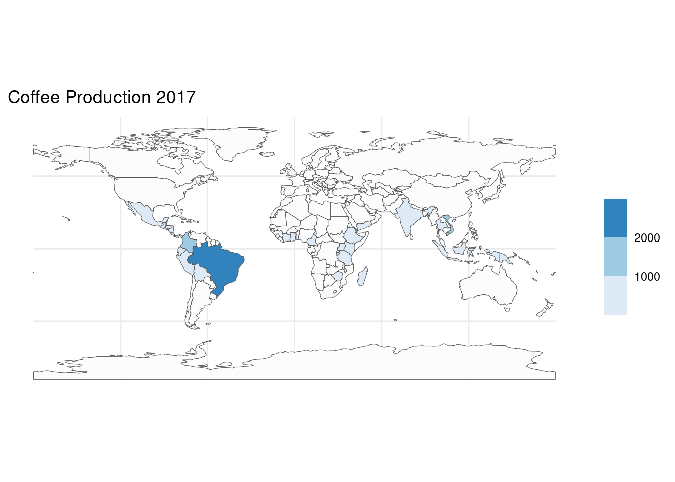
For joining to work, a ‘key variable’ must be supplied in both datasets. By default, dplyr uses all variables with matching names.
3.1.5 Creating and removing attributes
Often, we would like to create a new column based on already existing columns. For example, we want to calculate population density for each country.
world_new2 <- world |>
  mutate(pop_dens = pop / area_km2) |>
  select(name_long, pop_dens)

world_new2
## Simple feature collection with 177 features and 2 fields
## Geometry type: MULTIPOLYGON
## Dimension: XY
## Bounding box: xmin: -180 ymin: -89.9 xmax: 180 ymax: 83.64513
## Geodetic CRS: WGS 84
## # A tibble: 177 × 3
## name_long pop_dens geom
## <chr> <dbl> <MULTIPOLYGON [°]>
## 1 Fiji 45.9 (((-180 -16.55522, -179.9174 -16.50178, -179.7933 …
## 2 Tanzania 56.0 (((33.90371 -0.95, 31.86617 -1.02736, 30.76986 -1.…
## 3 Western Sahara NA (((-8.66559 27.65643, -8.817828 27.65643, -8.79488…
## 4 Canada 3.54 (((-132.71 54.04001, -133.18 54.16998, -133.2397 5…
## 5 United States 33.5 (((-171.7317 63.78252, -171.7911 63.40585, -171.55…
## 6 Kazakhstan 6.33 (((87.35997 49.21498, 86.82936 49.82667, 85.54127 …
## 7 Uzbekistan 66.7 (((55.96819 41.30864, 57.09639 41.32231, 56.93222 …
## 8 Papua New Guinea 16.7 (((141.0002 -2.600151, 141.0171 -5.859022, 141.033…
## 9 Indonesia 140. (((104.37 -1.084843, 104.0108 -1.059212, 103.4376 …
## 10 Argentina 15.4 (((-68.63401 -52.63637, -68.63335 -54.8695, -67.56…
## # ℹ 167 more rowsunite() from the tidyr package pastes together existing columns.
world_unite <- world |>
  tidyr::unite(col = "con_reg", continent:region_un, sep = ":", remove = TRUE) |>
  select(con_reg)

world_unite
## Simple feature collection with 177 features and 1 field
## Geometry type: MULTIPOLYGON
## Dimension: XY
## Bounding box: xmin: -180 ymin: -89.9 xmax: 180 ymax: 83.64513
## Geodetic CRS: WGS 84
## # A tibble: 177 × 2
## con_reg geom
## <chr> <MULTIPOLYGON [°]>
## 1 Oceania:Oceania (((-180 -16.55522, -179.9174 -16.50178, -179.7933 -16…
## 2 Africa:Africa (((33.90371 -0.95, 31.86617 -1.02736, 30.76986 -1.014…
## 3 Africa:Africa (((-8.66559 27.65643, -8.817828 27.65643, -8.794884 2…
## 4 North America:Americas (((-132.71 54.04001, -133.18 54.16998, -133.2397 53.8…
## 5 North America:Americas (((-171.7317 63.78252, -171.7911 63.40585, -171.5531 …
## 6 Asia:Asia (((87.35997 49.21498, 86.82936 49.82667, 85.54127 49.…
## 7 Asia:Asia (((55.96819 41.30864, 57.09639 41.32231, 56.93222 41.…
## 8 Oceania:Oceania (((141.0002 -2.600151, 141.0171 -5.859022, 141.0339 -…
## 9 Asia:Asia (((104.37 -1.084843, 104.0108 -1.059212, 103.4376 -0.…
## 10 South America:Americas (((-68.63401 -52.63637, -68.63335 -54.8695, -67.56244…
## # ℹ 167 more rowstidyr separate() splits one column into multiple columns using either a regular expression or character positions
world_separate <- world_unite |>
  tidyr::separate(con_reg, c("continent", "region_un"), sep = ":")

world_separate
## Simple feature collection with 177 features and 2 fields
## Geometry type: MULTIPOLYGON
## Dimension: XY
## Bounding box: xmin: -180 ymin: -89.9 xmax: 180 ymax: 83.64513
## Geodetic CRS: WGS 84
## # A tibble: 177 × 3
## continent region_un geom
## <chr> <chr> <MULTIPOLYGON [°]>
## 1 Oceania Oceania (((-180 -16.55522, -179.9174 -16.50178, -179.7933 -1…
## 2 Africa Africa (((33.90371 -0.95, 31.86617 -1.02736, 30.76986 -1.01…
## 3 Africa Africa (((-8.66559 27.65643, -8.817828 27.65643, -8.794884 …
## 4 North America Americas (((-132.71 54.04001, -133.18 54.16998, -133.2397 53.…
## 5 North America Americas (((-171.7317 63.78252, -171.7911 63.40585, -171.5531…
## 6 Asia Asia (((87.35997 49.21498, 86.82936 49.82667, 85.54127 49…
## 7 Asia Asia (((55.96819 41.30864, 57.09639 41.32231, 56.93222 41…
## 8 Oceania Oceania (((141.0002 -2.600151, 141.0171 -5.859022, 141.0339 …
## 9 Asia Asia (((104.37 -1.084843, 104.0108 -1.059212, 103.4376 -0…
## 10 South America Americas (((-68.63401 -52.63637, -68.63335 -54.8695, -67.5624…
## # ℹ 167 more rows![]()