3.2 Raster Objects

Raster data represent continuous surfaces across a grid pattern, often in multiple layers.

A tiff image is a raster data file.

Let’s build one from scratch.

The result is a raster object with 6 rows and 6 columns, and a minimum and maximum spatial extent in x and y direction. The vals argument sets the values that each cell contains: numeric data ranging from 1 to 36.

elev = rast(nrows = 6, ncols = 6,
            xmin = -1.5, xmax = 1.5, ymin = -1.5, ymax = 1.5,
            vals = 1:36)

plot(elev)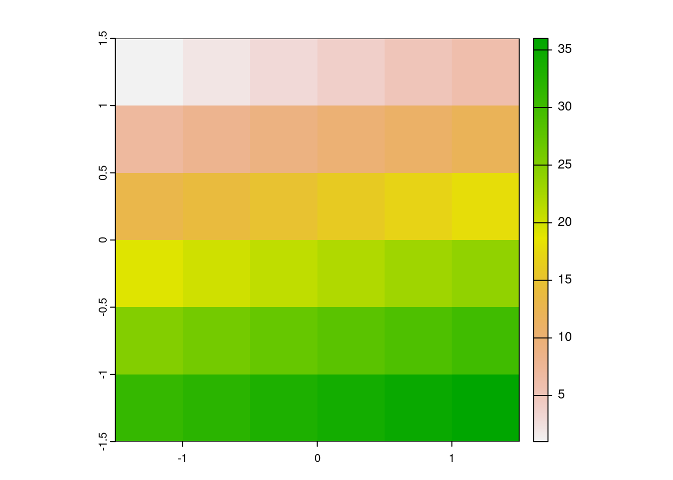

Raster objects can also contain categorical values of class logical or factor variables

grain_order <- c("clay", "silt", "sand")
grain_char <- sample(grain_order, 36, replace = TRUE)
grain_fact <- factor(grain_char, levels = grain_order)
grain <- rast(
  nrows = 6,
  ncols = 6,
  xmin = -1.5,
  xmax = 1.5,
  ymin = -1.5,
  ymax = 1.5,
  vals = grain_fact
)

plot(grain)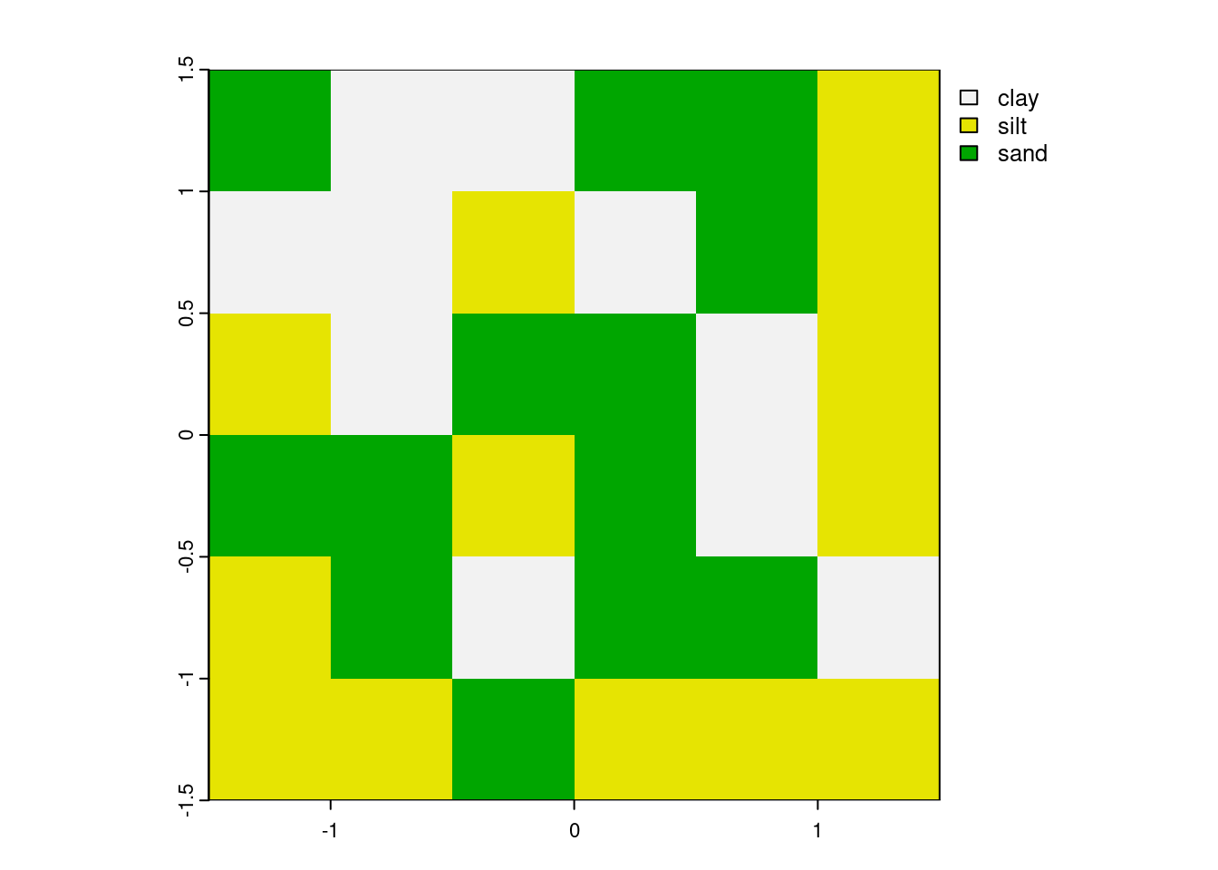

The raster object stores the corresponding look-up table as a list of data frames, which can be viewed with cats(grain)

3.2.1 Subsetting

In base R, [

elev[1,1]

##   lyr.1
## 1     1

Cell values can be modified by overwriting existing values in conjunction with a subsetting operation.

elev[3, 3] <- 0

elev[3, 3]

##   lyr.1
## 1     0

plot(elev)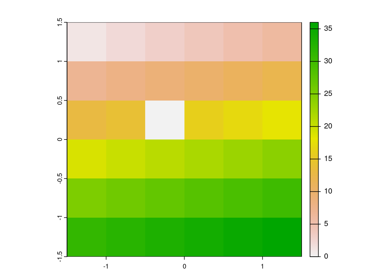

3.2.2 Summarizing

terra contains functions for extracting descriptive statistics for entire rasters.

summary operations such as the standard deviation or custom summary statistics can be calculated with global()

The freq() function allows to get the frequency table of categorical values.

elev

## class       : SpatRaster 
## dimensions  : 6, 6, 1  (nrow, ncol, nlyr)
## resolution  : 0.5, 0.5  (x, y)
## extent      : -1.5, 1.5, -1.5, 1.5  (xmin, xmax, ymin, ymax)
## coord. ref. : lon/lat WGS 84 
## source(s)   : memory
## name        : lyr.1 
## min value   :     0 
## max value   :    36

summary(elev)

##      lyr.1      
##  Min.   : 0.00  
##  1st Qu.: 8.75  
##  Median :18.50  
##  Mean   :18.08  
##  3rd Qu.:27.25  
##  Max.   :36.00

global(elev, sd)

##             sd
## lyr.1 10.96586

freq(elev)

##    layer value count
## 1      1     0     1
## 2      1     1     1
## 3      1     2     1
## 4      1     3     1
## 5      1     4     1
## 6      1     5     1
## 7      1     6     1
## 8      1     7     1
## 9      1     8     1
## 10     1     9     1
## 11     1    10     1
## 12     1    11     1
## 13     1    12     1
## 14     1    13     1
## 15     1    14     1
## 16     1    16     1
## 17     1    17     1
## 18     1    18     1
## 19     1    19     1
## 20     1    20     1
## 21     1    21     1
## 22     1    22     1
## 23     1    23     1
## 24     1    24     1
## 25     1    25     1
## 26     1    26     1
## 27     1    27     1
## 28     1    28     1
## 29     1    29     1
## 30     1    30     1
## 31     1    31     1
## 32     1    32     1
## 33     1    33     1
## 34     1    34     1
## 35     1    35     1
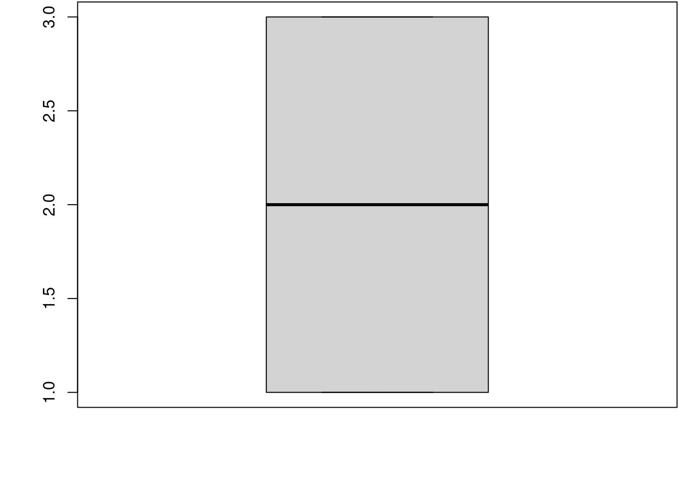
## 36     1    36     1

Raster value statistics can be visualized in a variety of ways. Specific functions such as boxplot(), density(), hist() and pairs() work also with raster objects.

par(mar = c(4, 4, .1, .1))

boxplot(grain)

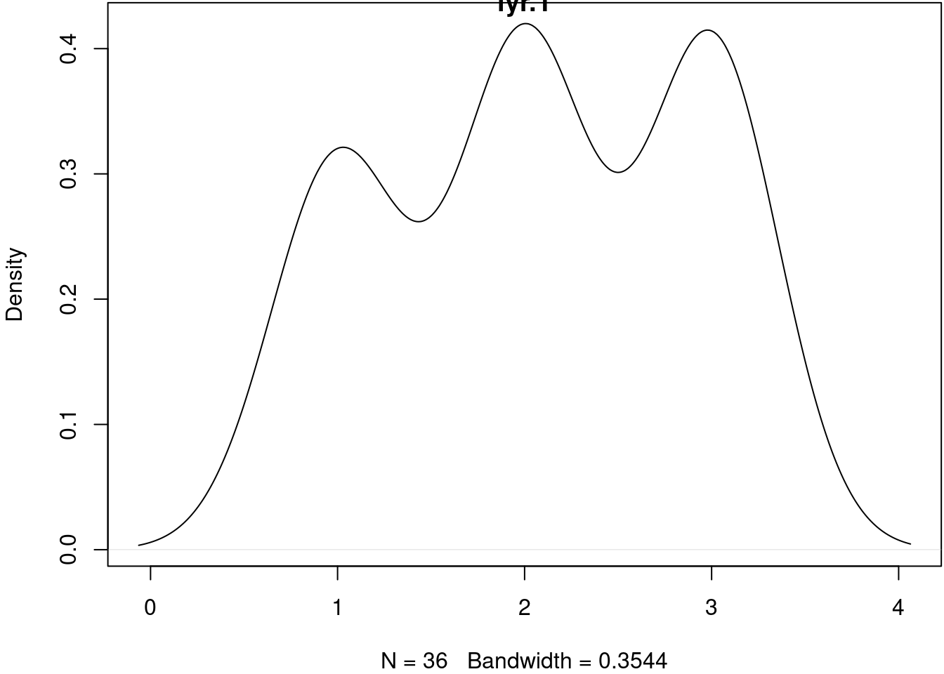
density(grain)

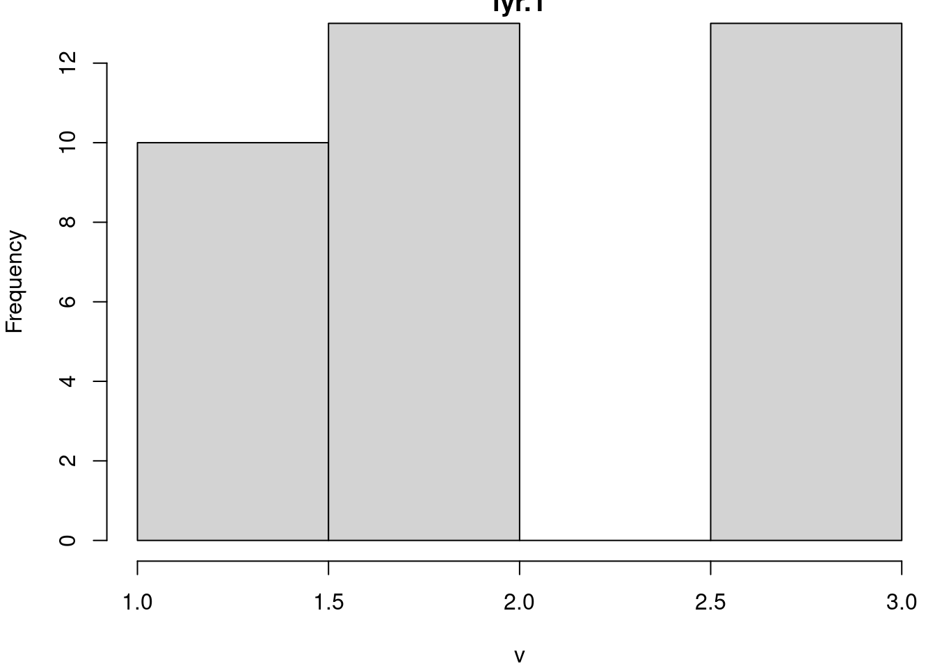
hist(grain)