13.6 Route Networks

Route networks are often also important outputs: summarizing data such as the potential number of trips made on particular segments can help prioritize investment where it is most needed.

An example:

Imagine that 50% of car trips between 0 to 3 km in route distance are replaced by cycling,a percentage that drops by 10 percentage points for every additional km of route distance so that 20% of car trips of 6 km are replaced by cycling and no car trips that are 8 km or longer are replaced by cycling.

The mode shift could be modeled as

uptake <- function(x) {
  case_when(
    x <= 3 ~ 0.5,
    x >= 8 ~ 0,
    TRUE ~ (8 - x) / (8 - 3) * 0.5
  )
}

routes_short_scenario <- routes_short |> 
  mutate(uptake = uptake(distance / 1000)) |> 
  mutate(bicycle = bicycle + car_driver * uptake,
         car_driver = car_driver * (1 - uptake))

sum(routes_short_scenario$bicycle) - sum(routes_short$bicycle)

## [1] 3790.963

Having created a scenario in which approximately 4000 trips have switched from driving to cycling, we can now model where this updated modeled cycling activity will take place.

overline breaks linestrings at junctions (were two or more linestring geometries meet), and calculates aggregate statistics for each unique route segment

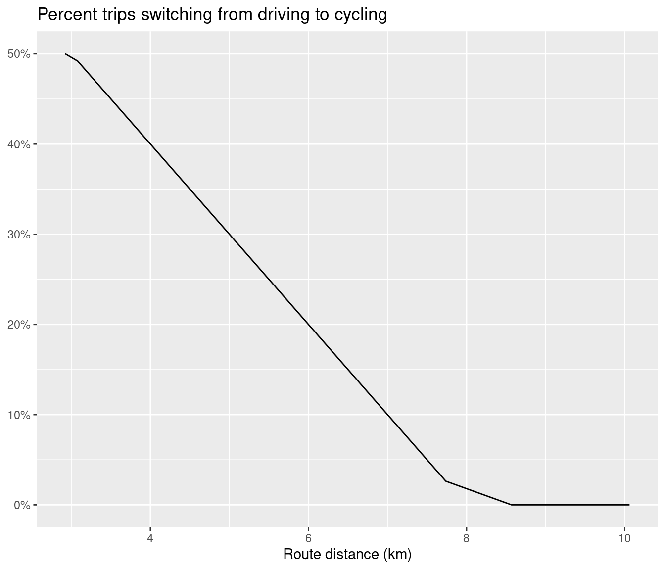
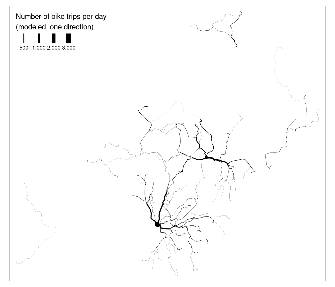
(#fig:13 mode shift illustated)Illustration of the percentage of car trips switching to cycling as a function of distance (left) and route network level results of this function (right).

Transport networks with records at the segment level, typically with attributes such as road type and width, constitute a common type of route network. Such route network datasets are available worldwide from OpenStreetMap.

We will use the author’s sample dataset bristol_ways, which represents just over 6000 segments.

summary(bristol_ways)

##      highway       maxspeed             ref                     geometry   
##  cycleway:1721   Length:6160        Length:6160        LINESTRING   :6160  
##  rail    :1017   Class :character   Class :character   epsg:4326    :   0  
##  road    :3422   Mode  :character   Mode  :character   +proj=long...:   0

sfnetworks offers igraph functionality, while preserving the geometric attributes

In the example below, the ‘edge betweenness’, meaning the number of shortest paths passing through each edge, is calculated.

ways_sfn <- as_sfnetwork(bristol_ways)
class(ways_sfn)

## [1] "sfnetwork" "tbl_graph" "igraph"

ways_centrality <- ways_sfn |> 
  sfnetworks::activate("edges") |>  
  mutate(betweenness = tidygraph::centrality_edge_betweenness())  # removed the "length" param from the book

bb_wayssln = tmaptools::bb(route_network_scenario, xlim = c(0.1, 0.9), ylim = c(0.1, 0.6), relative = TRUE)

tm_shape(ways_centrality |> 
           st_as_sf(), bb = bb_wayssln) +
  tm_lines(lwd = "betweenness", scale = 9, title.lwd = "Betweenness", col = "grey",
    lwd.legend = c(5000, 10000), legend.lwd.is.portrait = TRUE) +
  tm_shape(route_network_scenario) +
  tm_lines(lwd = "bicycle", scale = 9, title.lwd = "Number of bike trips (modeled, one direction)",
    lwd.legend = c(1000, 2000), legend.lwd.is.portrait = TRUE, col = "darkgreen")

The results demonstrate that each graph edge represents a segment: the segments near the center of the road network have the highest betweenness values, whereas segments closer to central Bristol have higher cycling potential, based on these simplistic datasets.

One can also find the shortest route between origins and destinations using this graph representation of the route network with the sfnetworks package.

The example dataset we used above is relatively small. It may also be worth considering how the work could adapt to larger networks