13.5 Routes

We will add an additional layer of complexity by considering the built infrastructure.

Routing engines can be multi-modal, or not. Transit policy studies really must be multi-modal. They generate routes (a multi-linestring geometry for each trip), legs (each mode within the route), and segments (an OpenStreetMap turn by turn event list).

The more detail, the larger the file size.

In-memory routing

Routing engines in R enable route networks stored as R objects in memory to be used as the basis of route calculation. Options include sfnetworks, dodgr and cppRouting packages.

While fast and flexible, native R routing options are generally harder to set-up than dedicated routing engines for realistic route calculation. Routing is a hard problem and many hundreds of hours have been put into open source routing engines that can be downloaded and hosted locally. On the other hand, R-based routing engines may be well-suited to model experiments and the statistical analysis of the impacts of changes on the network. Changing route network characteristics (or weights associated with different route segment types), re-calculating routes, and analyzing results under many scenarios in a single language has benefits for research applications.

Locally hosted dedicated routing engines

Locally hosted routing engines include OpenTripPlanner, Valhalla, and R5 (which are multi-modal), and the OpenStreetMap Routing Machine (OSRM) (which is ‘uni-modal’). These can be accessed from R with the packages opentripplanner, valhalla, r5r and osrm (Morgan et al. 2019; Pereira et al. 2021). Locally hosted routing engines run on the user’s computer but in a process separate from R. They benefit from speed of execution and control over the weighting profile for different modes of transport. Disadvantages include the difficulty of representing complex networks locally; temporal dynamics (primarily due to traffic); and the need for specialized external software.

Remotely hosted dedicated routing engines

Remotely hosted routing engines use a web API to send queries about origins and destinations and return results. Routing services based on open source routing engines, such as OSRM’s publicly available service, work the same when called from R as locally hosted instances, simply requiring arguments specifying ‘base URLs’ to be updated.

Advantages: - Provision of routing services worldwide (or usually at least over a large region) - Established routing services available are usually update regularly and can often respond to traffic levels - Routing services usually run on dedicated hardware and software including systems such as load balancers to ensure consistent performance

Disadvantages - cost - web connectivity requirement

A worked example:

Cycling is most beneficial when it replaces car trips. Let’s isolate them with a filter on st_length the length of the desire line. Then we will call the stplanr route() function to generate an sf object that represents the portion of the network that are suitable for cycling, one for each desire line, calling the osrm API.

We then plot desire lines along which many short car journeys take place alongside cycling routes.

desire_lines <- desire_lines |> 
  mutate(distance_km = as.numeric(st_length(desire_lines))/ 1000)

desire_lines_short <- desire_lines |> 
  filter(car_driver >= 100, distance_km <= 5, distance_km >= 2.5)

routes_short <- route(l = desire_lines_short, 
                      route_fun = route_osrm,
                     osrm.profile = "bike")

## Most common output is sf

routes_plot_data <- rbind(
  desire_lines_short |> transmute(Entity = "Desire lines") |> sf::st_set_crs("EPSG:4326"),
  routes_short |> transmute(Entity = "Cycling Routes") |> sf::st_set_crs("EPSG:4326")
)

zone_cents_routes <- zone_cents[desire_lines_short, ]

## although coordinates are longitude/latitude, st_intersects assumes that they
## are planar

routes_plot_data |> 
  ggplot() +
  geom_sf(aes(color = Entity, linetype = Entity)) +
  scale_color_manual(values = c("black", "red")) +
  scale_linetype_manual(values = c(2, 1)) +
  geom_sf(data = zone_cents_routes) +
  theme_void()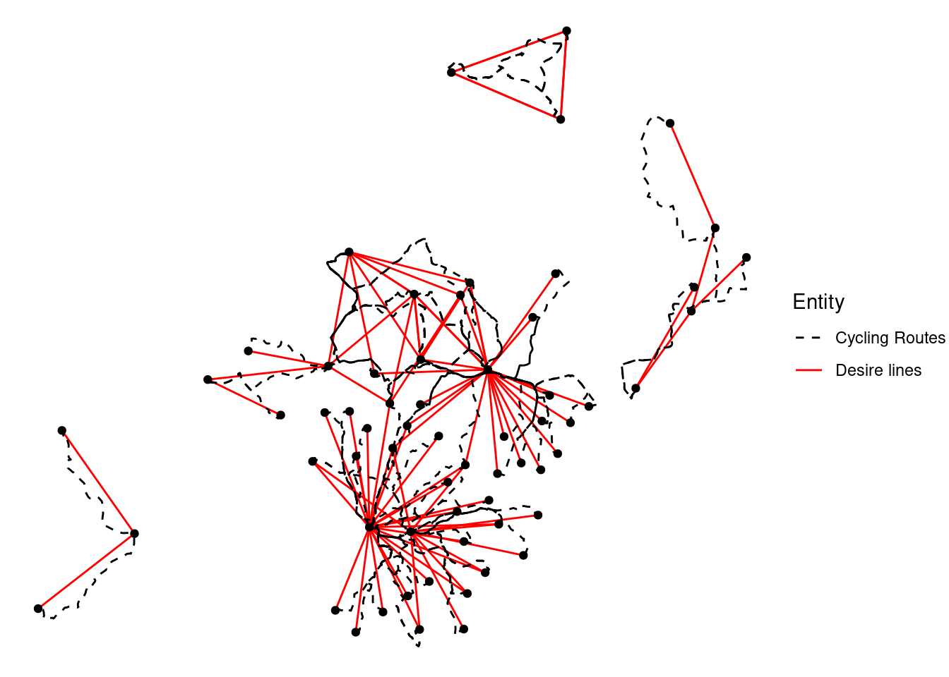

There are many benefits of converting travel desire lines into routes.

It is important to remember that we cannot be sure how many (if any) trips will follow the exact routes calculated by routing engines. However, route and street/way/segment level results can be highly policy relevant.