13.3 Desire Lines

Desire lines connect origins and destinations, representing where people desire to go, typically between zones. They are often represented conveniently using zone centroids. Let’s just use the top 10:

(od_top10 <- bristol_od |> 
  dplyr::slice_max(all, n = 10))

## # A tibble: 10 × 7
##    o         d           all bicycle  foot car_driver train
##    <chr>     <chr>     <dbl>   <dbl> <dbl>      <dbl> <dbl>
##  1 E02003043 E02003043  1493      66  1296         64     8
##  2 E02003047 E02003043  1300     287   751        148     8
##  3 E02003031 E02003043  1221     305   600        176     7
##  4 E02003037 E02003043  1186      88   908        110     3
##  5 E02003034 E02003043  1177     281   711        100     7
##  6 E02003027 E02003043  1166     311   357        262     6
##  7 E02003036 E02003043  1099     115   868         54     5
##  8 E02003033 E02003043  1093     120   802        110     5
##  9 E02003019 E02003019   990      72   331        493     3
## 10 E02003050 E02003043   958     126   585        113     5

Walking is the most popular mode of transport among the top pairs

E02003043 is a popular destination (city center)

Also, intrazonal city center is number one

he percentage of each desire line that is made by these active modes:

(bristol_od <- bristol_od |> 
  mutate(Active = (bicycle + foot) / all * 100))

## # A tibble: 2,910 × 8
##    o         d           all bicycle  foot car_driver train Active
##    <chr>     <chr>     <dbl>   <dbl> <dbl>      <dbl> <dbl>  <dbl>
##  1 E02002985 E02002985   209       5   127         59     0  63.2 
##  2 E02002985 E02002987   121       7    35         62     0  34.7 
##  3 E02002985 E02003036    32       2     1         10     1   9.38
##  4 E02002985 E02003043   141       1     2         56    17   2.13
##  5 E02002985 E02003049    56       2     4         36     0  10.7 
##  6 E02002985 E02003054    42       4     0         21     0   9.52
##  7 E02002985 E02003100    22       0     0         19     3   0   
##  8 E02002985 E02003106    48       3     1         33     8   8.33
##  9 E02002985 E02003108    31       0     0         29     1   0   
## 10 E02002985 E02003121    42       1     2         34     0   7.14
## # ℹ 2,900 more rows

Let’s separate interzonal from intrazonal

od_intra <- dplyr::filter(bristol_od, o == d)
od_inter <- dplyr::filter(bristol_od, o != d)

The next step is to convert the interzonal OD pairs into an sf object

For real-world use one should use centroid values generated from projected data or, preferably, use population-weighted centroids

desire_lines <- od2line(od_inter, zones_od) # creates centroids

## Creating centroids representing desire line start and end points.

desire_lines_top10 <- od2line(od_top10, zones_od)

## Creating centroids representing desire line start and end points.

tm_shape(desire_lines) +
  tm_lines(palette = "plasma", breaks = c(0, 5, 10, 20, 40, 100),
    lwd = "all",
    scale = 9,
    title.lwd = "Number of trips",
    alpha = 0.1,           # lightened to help emphasize the top 10
    col = "Active",
    title = "Active travel (%)"
  ) +
  tm_shape(desire_lines_top10) +
  tm_lines(lwd = 5, col = "green", alpha = 0.7) +
  tm_scale_bar()

## Legend labels were too wide. Therefore, legend.text.size has been set to 0.61. Increase legend.width (argument of tm_layout) to make the legend wider and therefore the labels larger.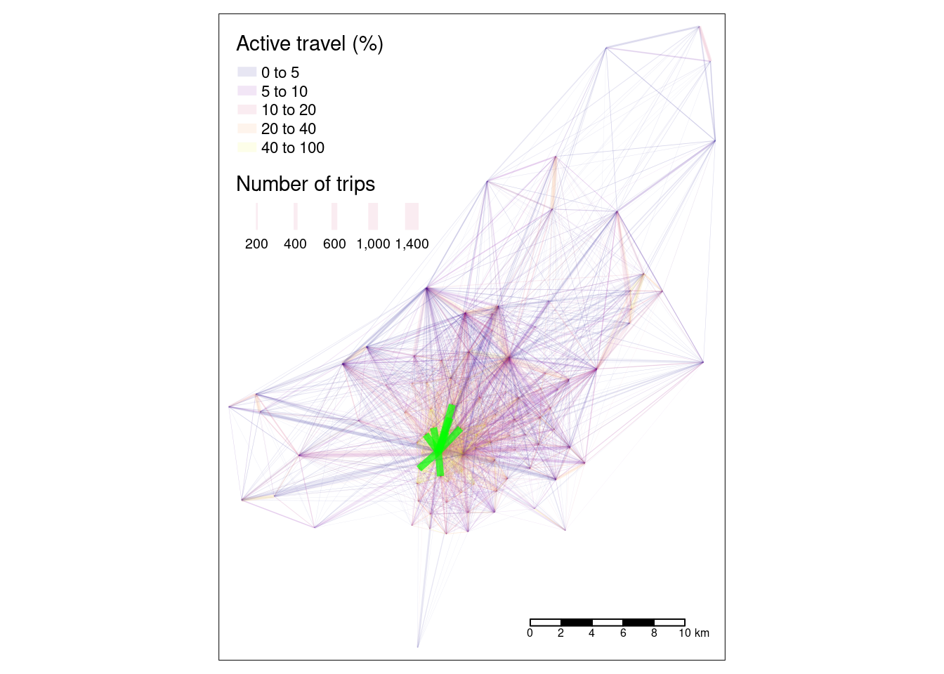

The map shows that the city center dominates transport patterns in the region, suggesting policies should be prioritized there, although a number of peripheral sub-centers can also be seen.