13.2 Transport Zones

Two zone types are of particular interest to transport researchers: origin and destination zones

Different zoning systems, such as ‘Workplace Zones’, may be appropriate to represent the increased density of trip destinations in areas with many ‘trip attractors’ such as schools and shops.

Travel to Work Areas (TTWAs) create a zoning system analogous to hydrological watersheds.

There are 102 TTWA zones in our dataset.

bristol_od has more rows than bristol_zones because it represents travel between zones

The o column is origin and the d is destination

nrow(bristol_od)

## [1] 2910

names(bristol_od)

## [1] "o"          "d"          "all"        "bicycle"    "foot"      
## [6] "car_driver" "train"

nrow(bristol_zones)

## [1] 102

zones_attr <- bristol_od |> 
  group_by(o) |> 
  summarize(across(where(is.numeric), sum)) |> 
  dplyr::rename(geo_code = o)

zones_attr

## # A tibble: 102 × 6
##    geo_code    all bicycle  foot car_driver train
##    <chr>     <dbl>   <dbl> <dbl>      <dbl> <dbl>
##  1 E02002985   868      30   173        414    43
##  2 E02002987   898      34   117        523    58
##  3 E02003005   786      19    91        593     8
##  4 E02003012  3312     161   330       2058    12
##  5 E02003013  3715     188   615       2021     6
##  6 E02003014  2220     126   270       1239     5
##  7 E02003015  1633     166   307        786     7
##  8 E02003016  2411     218   440       1105    23
##  9 E02003017  1590     187   208        898     9
## 10 E02003018  1690      96   143       1048    20
## # ℹ 92 more rows

zones_joined <- bristol_zones |> 
    left_join(zones_attr, by = "geo_code")

sum(zones_joined$all)

## [1] 238805

names(zones_joined)

## [1] "geo_code"   "name"       "all"        "bicycle"    "foot"      
## [6] "car_driver" "train"      "geometry"

The result contains columns representing the total number of trips originating in each zone and their mode of travel (by bicycle, foot, car and train).

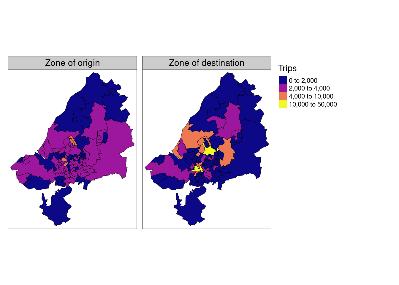
Most zones have between 0 and 4,000 trips originating from them.

Low trip numbers in the outskirts of the region might be explained by the fact that many people in these peripheral zones will travel to other regions outside of the study area.

zones_destinations <- bristol_od |> 
  group_by(d) |> 
  summarize(across(where(is.numeric), sum)) |> 
  select(geo_code = d, all_dest = all)

zones_od = zones_joined |> 
  inner_join(zones_destinations, by = "geo_code")

tm_shape(zones_od) +
  tm_fill(
    c("all", "all_dest"),
    palette = viridis::plasma(4),
    breaks = c(0, 2000, 4000, 10000, 50000),
    title = "Trips"
  )  +
  tm_borders(col = "black", lwd = 0.5) +
  tm_facets(free.scales = FALSE, ncol = 2) +
  tm_layout(panel.labels = c("Zone of origin", "Zone of destination"))