12.3 Supervised Learning
We fit a logistic regression model through the generalized linear models tools.
glm_fit = glm(lslpts ~ slope + cplan + cprof + elev + log10_carea,
          family = binomial(), #logistic regression
          data = lsl)

summary(glm_fit)
##
## Call:
## glm(formula = lslpts ~ slope + cplan + cprof + elev + log10_carea,
## family = binomial(), data = lsl)
##
## Coefficients:
## Estimate Std. Error z value Pr(>|z|)
## (Intercept) 2.511e+00 2.035e+00 1.234 0.217
## slope 7.901e-02 1.506e-02 5.248 1.54e-07 ***
## cplan -2.894e+01 4.746e+00 -6.098 1.07e-09 ***
## cprof -1.756e+01 1.083e+01 -1.622 0.105
## elev 1.789e-04 5.492e-04 0.326 0.745
## log10_carea -2.275e+00 4.848e-01 -4.692 2.70e-06 ***
## ---
## Signif. codes: 0 '***' 0.001 '**' 0.01 '*' 0.05 '.' 0.1 ' ' 1
##
## (Dispersion parameter for binomial family taken to be 1)
##
## Null deviance: 485.20 on 349 degrees of freedom
## Residual deviance: 372.83 on 344 degrees of freedom
## AIC: 384.83
##
## Number of Fisher Scoring iterations: 4Next, we can predict various levels of landslide susceptibility
glm_pred = predict(object = glm_fit, type = "response")
summary(glm_pred)
## Min. 1st Qu. Median Mean 3rd Qu. Max.
## 0.002336 0.267687 0.523871 0.500000 0.724572 0.985877Here, we visualize the predictions
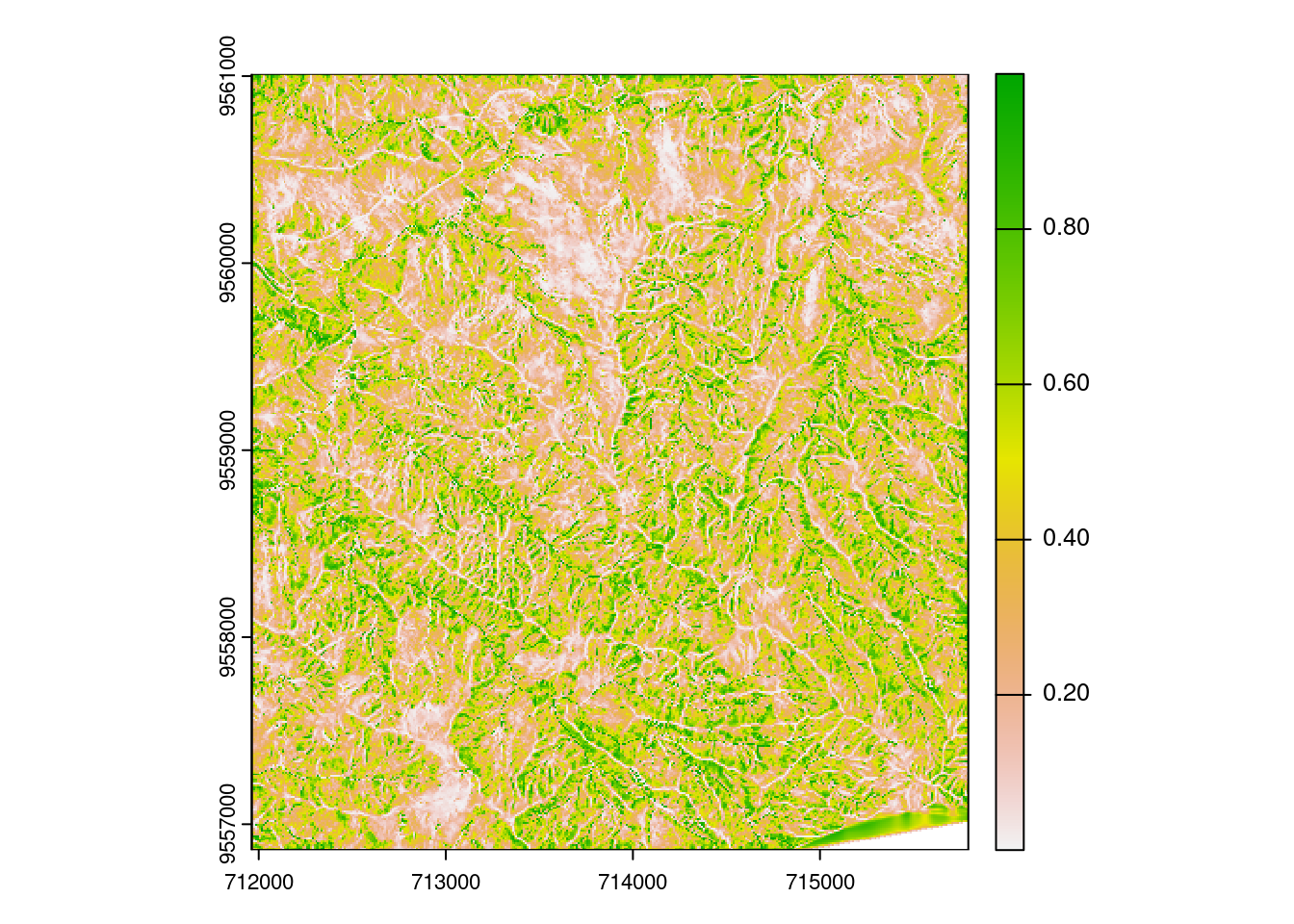
glm_pred_rast = terra::predict(ta, model = glm_fit, type = "response")
plot(glm_pred_rast)
12.3.1 AUROC
The most popular measure to assess the predictive performance of a binomial model is the Area Under the Receiver Operator Characteristic Curve (AUROC). This is a value between 0.5 and 1.0, with 0.5 indicating a model that is no better than random and 1.0 indicating perfect prediction of the two classes. Thus, the higher the AUROC, the better the model’s predictive power.
pROC::auc(pROC::roc(lsl$lslpts, fitted(glm_fit)))## Area under the curve: 0.8216