Chapter 15 Ecology
Abstract
This chapter models the floristic gradient of fog oases to reveal distinctive vegetation belts that are clearly controlled by water availability. The case study provides an opportunity to bring together and extend concepts presented in previous chapters to further enhance your skills at using R for geocomputation.
Fog oases, locally called lomas, are vegetation formations found on mountains along the coastal deserts of Peru and Chile. Similar ecosystems can be found elsewhere, including in the deserts of Namibia and along the coasts of Yemen and Oman (Galletti, Turner, and Myint 2016). Despite the arid conditions and low levels of precipitation of around 30-50 mm per year on average, fog deposition increases the amount of water available to plants during austral winter, resulting in green southern-facing mountain slopes along the coastal strip of Peru. The fog, which develops below the temperature inversion caused by the cold Humboldt current in austral winter, provides the name for this habitat. Every few years, the El Niño phenomenon brings torrential rainfall to this sun-baked environment, providing tree seedlings a chance to develop roots long enough to survive the following arid conditions (Dillon, Nakazawa, and Leiva 2003).
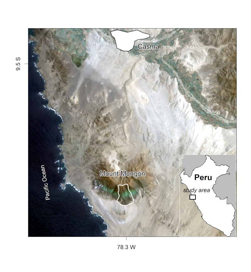
Unfortunately, fog oases are heavily endangered, primarily due to agriculture and anthropogenic climate change. Evidence on the composition and spatial distribution of the native flora can support efforts to protect remaining fragments of fog oases (Muenchow, Bräuning, et al. 2013; Muenchow, Hauenstein, et al. 2013). The chapter also demonstrates how to apply techniques covered in previous chapters to an important applied field: ecology.In it you will analyze the composition and the spatial distribution of vascular plants (here referring mostly to flowering plants) on the southern slope of Mt. Mongón, a lomas mountain near Casma on the central northern coast of Peru

southern slope of Mt Mongón
Methods
During a field study to Mt. Mongón, all vascular plants living in 100 randomly sampled 4x4 m2 plots in the austral winter of 2011 were recorded(Muenchow, Bräuning, et al. 2013). The sampling coincided with a strong La Niña event that year, as shown in data published by the National Oceanic and Atmospheric Administration (NOAA). This led to even higher levels of aridity than usual in the coastal desert and increased fog activity on the southern slopes of Peruvian lomas mountains.For this, we will make use of a random forest model — a very popular machine learning algorithm (Breiman 2001). The model will allow us to make spatial distribution maps of the floristic composition anywhere in the study area.
library("data.table") # fast data.frame manipulation (used by mlr3)##
## Attaching package: 'data.table'## The following objects are masked from 'package:lubridate':
##
## hour, isoweek, mday, minute, month, quarter, second, wday, week,
## yday, year## The following object is masked from 'package:purrr':
##
## transpose## The following objects are masked from 'package:dplyr':
##
## between, first, last## The following object is masked from 'package:terra':
##
## shiftlibrary("dplyr")
library("mlr3") # machine learning (see Chapter 12)
library("mlr3spatiotempcv") # spatio-temporal resampling
library("mlr3tuning") # hyperparameter tuning package
library("mlr3learners") # interface to most important machine learning packages
library("paradox") # defining hyperparameter spaces
# library("qgisprocess") # bridge to QGIS (Chapter 10)
library("ranger") # random forest package
library("sf")
library("terra")
library("tree") # decision tree package
library("vegan") # community ecology package## Loading required package: permute## Loading required package: lattice## This is vegan 2.6-4sessionInfo()## R version 4.3.1 (2023-06-16)
## Platform: x86_64-pc-linux-gnu (64-bit)
## Running under: Ubuntu 22.04.2 LTS
##
## Matrix products: default
## BLAS: /usr/lib/x86_64-linux-gnu/openblas-pthread/libblas.so.3
## LAPACK: /usr/lib/x86_64-linux-gnu/openblas-pthread/libopenblasp-r0.3.20.so; LAPACK version 3.10.0
##
## locale:
## [1] LC_CTYPE=C.UTF-8 LC_NUMERIC=C LC_TIME=C.UTF-8
## [4] LC_COLLATE=C.UTF-8 LC_MONETARY=C.UTF-8 LC_MESSAGES=C.UTF-8
## [7] LC_PAPER=C.UTF-8 LC_NAME=C LC_ADDRESS=C
## [10] LC_TELEPHONE=C LC_MEASUREMENT=C.UTF-8 LC_IDENTIFICATION=C
##
## time zone: UTC
## tzcode source: system (glibc)
##
## attached base packages:
## [1] grid stats graphics grDevices utils datasets methods
## [8] base
##
## other attached packages:
## [1] vegan_2.6-4 lattice_0.21-8 permute_0.9-7
## [4] tree_1.0-43 ranger_0.15.1 data.table_1.14.8
## [7] osmdata_0.2.3 sfnetworks_0.6.3 stplanr_1.0.2
## [10] progressr_0.13.0 pROC_1.18.2 mlr3viz_0.6.1
## [13] mlr3tuning_0.18.0 paradox_0.11.1 mlr3spatiotempcv_2.1.0
## [16] mlr3learners_0.5.6 mlr3_0.16.1 lgr_0.4.4
## [19] future_1.32.0 tmap_3.3-3 mapview_2.11.0
## [22] leaflet_2.1.2 colorspace_2.1-0 lubridate_1.9.2
## [25] forcats_1.0.0 stringr_1.5.0 purrr_1.0.1
## [28] readr_2.1.4 tibble_3.2.1 tidyverse_2.0.0
## [31] ggplot2_3.4.2 tidyr_1.3.0 dplyr_1.1.2
## [34] sp_2.0-0 spDataLarge_2.0.9 spData_2.2.2
## [37] terra_1.7-37 sf_1.0-13
##
## loaded via a namespace (and not attached):
## [1] RColorBrewer_1.1-3 rstudioapi_0.14 jsonlite_1.8.5
## [4] wk_0.7.3 magrittr_2.0.3 farver_2.1.1
## [7] rmarkdown_2.22 vctrs_0.6.3 base64enc_0.1-3
## [10] webshot_0.5.4 htmltools_0.5.5 leafsync_0.1.0
## [13] curl_5.0.1 raster_3.6-20 s2_1.1.4
## [16] sass_0.4.6 parallelly_1.36.0 KernSmooth_2.23-21
## [19] bslib_0.5.0 htmlwidgets_1.6.2 plyr_1.8.8
## [22] palmerpenguins_0.1.1 stars_0.6-1 cachem_1.0.8
## [25] uuid_1.1-0 igraph_1.5.0 lifecycle_1.0.3
## [28] pkgconfig_2.0.3 Matrix_1.5-4.1 R6_2.5.1
## [31] fastmap_1.1.1 digest_0.6.31 GGally_2.1.2
## [34] reshape_0.8.9 mlr3misc_0.12.0 leafem_0.2.0
## [37] crosstalk_1.2.0 labeling_0.4.2 lwgeom_0.2-13
## [40] fansi_1.0.4 timechange_0.2.0 mgcv_1.8-42
## [43] abind_1.4-5 compiler_4.3.1 proxy_0.4-27
## [46] bit64_4.0.5 withr_2.5.0 brew_1.0-8
## [49] backports_1.4.1 viridis_0.6.3 DBI_1.1.3
## [52] highr_0.10 MASS_7.3-60 tmaptools_3.1-1
## [55] classInt_0.4-9 tools_4.3.1 units_0.8-2
## [58] geodata_0.5-8 glue_1.6.2 satellite_1.0.4
## [61] nlme_3.1-162 checkmate_2.2.0 cluster_2.1.4
## [64] generics_0.1.3 gtable_0.3.3 leaflet.providers_1.9.0
## [67] tzdb_0.4.0 class_7.3-22 nabor_0.5.0
## [70] hms_1.1.3 tidygraph_1.2.3 utf8_1.2.3
## [73] pillar_1.9.0 vroom_1.6.3 splines_4.3.1
## [76] bbotk_0.7.2 bit_4.0.5 tidyselect_1.2.0
## [79] pbapply_1.7-0 sfheaders_0.4.3 knitr_1.43
## [82] gridExtra_2.3 bookdown_0.34 svglite_2.1.1
## [85] stats4_4.3.1 xfun_0.39 leafpop_0.1.0
## [88] stringi_1.7.12 yaml_2.3.7 evaluate_0.21
## [91] codetools_0.2-19 cli_3.6.1 tidyterra_0.4.0
## [94] systemfonts_1.0.4 munsell_0.5.0 jquerylib_0.1.4
## [97] dichromat_2.0-0.1 Rcpp_1.0.10 globals_0.16.2
## [100] png_0.1-8 XML_3.99-0.14 parallel_4.3.1
## [103] ellipsis_0.3.2 listenv_0.9.0 viridisLite_0.4.2
## [106] scales_1.2.1 e1071_1.7-13 crayon_1.5.2
## [109] rlang_1.1.1 mlr3measures_0.5.0