12.9 Tuning
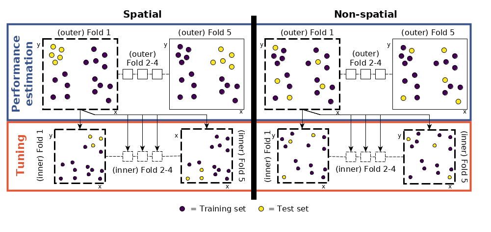
The next step is new, however: to tune the hyperparameters. Using the same data for the performance assessment and the tuning would potentially lead to overoptimistic results (Cawley and Talbot 2010). This can be avoided using nested spatial CV. [Figure was taken from Schratz et al. (2019)]
nested spatial CV
# five spatially disjoint partitions
tune_level = mlr3::rsmp("spcv_coords", folds = 5)
# use 50 randomly selected hyperparameters
terminator = mlr3tuning::trm("evals", n_evals = 50)
tuner = mlr3tuning::tnr("random_search")
# define the outer limits of the randomly selected hyperparameters
search_space = paradox::ps(
  C = paradox::p_dbl(lower = -12, upper = 15, trafo = function(x) 2^x),
  sigma = paradox::p_dbl(lower = -15, upper = 6, trafo = function(x) 2^x)
)
at_ksvm = mlr3tuning::AutoTuner$new(
learner = lrn_svm,
resampling = tune_level,
measure = mlr3::msr("classif.auc"),
search_space = search_space,
terminator = terminator,
tuner = tuner
)Accounting
The tuning is now set-up to fit 250 models to determine optimal hyperparameters for one fold. Repeating this for each fold, we end up with 1,250 (250 * 5) models for each repetition. Repeated 100 times means fitting a total of 125,000 models to identify optimal hyperparameters (Figure 12.3). These are used in the performance estimation, which requires the fitting of another 500 models (5 folds * 100 repetitions; see Figure 12.3). To make the performance estimation processing chain even clearer, let us write down the commands we have given to the computer:
- Performance level (upper left part of Figure 12.6) - split the dataset into five spatially disjoint (outer) subfolds
- Tuning level (lower left part of Figure 12.6) - use the first fold of the performance level and split it again spatially into five (inner) subfolds for the hyperparameter tuning. Use the 50 randomly selected hyperparameters in each of these inner subfolds, i.e., fit 250 models
- Performance estimation - Use the best hyperparameter combination from the previous step (tuning level) and apply it to the first outer fold in the performance level to estimate the performance (AUROC)
- Repeat steps 2 and 3 for the remaining four outer folds
- Repeat steps 2 to 4, 100 times
The process of hyperparameter tuning and performance estimation is computationally intensive.
# execute the outer loop sequentially and parallelize the inner loop
future::plan(list("sequential", "multisession"),
             workers = floor(availableCores() / 2))
# CAUTION: "It can easily run for half a day on a modern laptop."
progressr::with_progress(expr = {
rr_spcv_svm = mlr3::resample(task = task,
learner = at_ksvm,
# outer resampling (performance level)
resampling = perf_level,
store_models = FALSE,
encapsulate = "evaluate")
})
# stop parallelization
future:::ClusterRegistry("stop")
# compute the AUROC values
score_spcv_svm = rr_spcv_svm$score(measure = mlr3::msr("classif.auc"))
# keep only the columns you need
score_spcv_svm = score_spcv_svm[, .(task_id, learner_id, resampling_id, classif.auc)]score = readRDS("extdata/12-bmr_score.rds")
score_spcv_svm = score[learner_id == "classif.ksvm.tuned" &
resampling_id == "repeated_spcv_coords"]
# final mean AUROC
round(mean(score_spcv_svm$classif.auc), 2)## [1] 0.74