10.3 Resampling methods

This diagram from the Hands-on machine learning in R from Boehmke & Greenwell illustrates how resampling fits into the general modeling workflow:

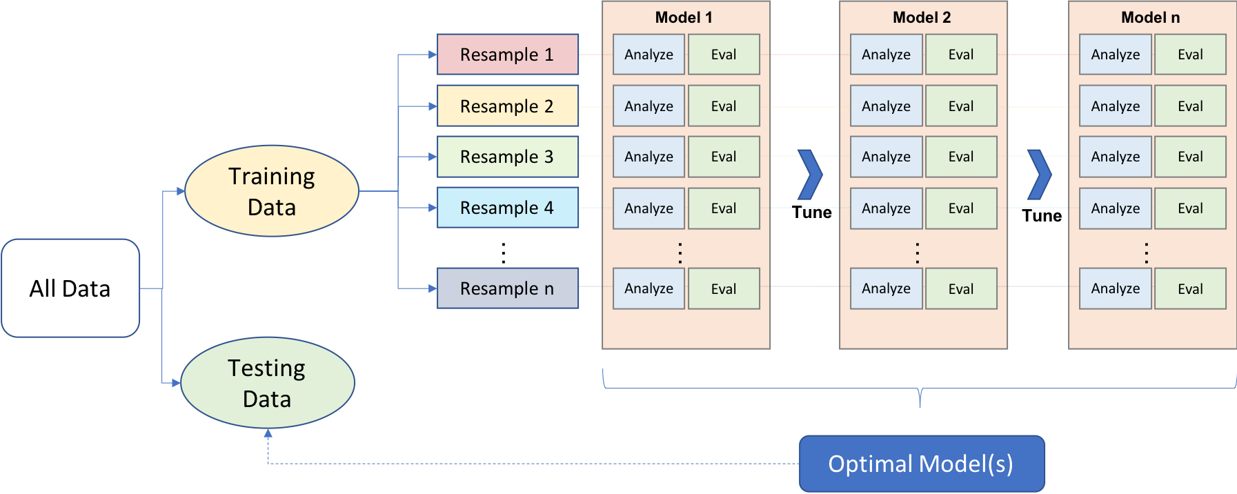
We can see that in resampling:

- happens after the data split into training and test sets

- some data is used for analyzing (analysis set), and some for evaluation (evaluation or assessment set, we’ll use assessment set from now on)

- this is an iterative as it can be repeated many times - it only applies to the training data

Effectively,

- the model is fit with the analysis set

- the model is evaluated with the evaluation set

The overall, final performance evaluation for the model is the average of the performance metrics of the n evaluation sets.

The way in which these analysis and evaluation sets are created define what the resampling techniques are specifically. We’ll go through the common ones:

cross-validation
repeated cross-validation
leave-one-out cross-validation
monte-carlo cross-validation

10.3.1 Cross-validation

Cross-validation is one of the most popular resampling techniques. There are several flavors

10.3.1.1 V-fold cross-validation

V-fold cross-validation involves the random splitting of the training data into approximately equal-sized “folds”. The diagram below illustrates v-fold cross validation with v set to 3 folds.

We can see that the training data points have been randomly assigned to roughly equal-sized folds (in this case, exactly equal) and that the assessment set for each fold is 2/3 of the training data. Max and Julia note that while 3-fold CV is good to use for illustrative purposed, it is not good in practice - in practice, rather 5- or 10- fold CV is preferred.

set.seed(55)
ames_folds <- vfold_cv(ames_train, v = 10)
ames_folds

## #  10-fold cross-validation 
## # A tibble: 10 × 2
##    splits             id    
##    <list>             <chr> 
##  1 <split [2107/235]> Fold01
##  2 <split [2107/235]> Fold02
##  3 <split [2108/234]> Fold03
##  4 <split [2108/234]> Fold04
##  5 <split [2108/234]> Fold05
##  6 <split [2108/234]> Fold06
##  7 <split [2108/234]> Fold07
##  8 <split [2108/234]> Fold08
##  9 <split [2108/234]> Fold09
## 10 <split [2108/234]> Fold10

The output contains info on how the training data was split: ~2000 are in the analysis set, and ~220 are in the assessment set. You can recuperate these sets by calling analysis() or assessment().

In chapter 5, we introduced the idea of stratified sampling, which is almost always useful but particularly in cases with class imbalance. You can perform V-fold CV with stratified samplying by using the strata argument in the vfold_cv() call.

10.3.1.2 Repeated cross validation

V-fold CV introduced above may produce noisy estimates. A technique that averages over more than V statistics may be more appropriate to reduce the noise. This technique is repeated cross-validation, where we create R repeats of V-fold CV. Instead of averaging over V statistics, we are now averaging over V x R statistics:

vfold_cv(ames_train, v = 10, repeats = 5)

## #  10-fold cross-validation repeated 5 times 
## # A tibble: 50 × 3
##    splits             id      id2   
##    <list>             <chr>   <chr> 
##  1 <split [2107/235]> Repeat1 Fold01
##  2 <split [2107/235]> Repeat1 Fold02
##  3 <split [2108/234]> Repeat1 Fold03
##  4 <split [2108/234]> Repeat1 Fold04
##  5 <split [2108/234]> Repeat1 Fold05
##  6 <split [2108/234]> Repeat1 Fold06
##  7 <split [2108/234]> Repeat1 Fold07
##  8 <split [2108/234]> Repeat1 Fold08
##  9 <split [2108/234]> Repeat1 Fold09
## 10 <split [2108/234]> Repeat1 Fold10
## # ℹ 40 more rows

10.3.1.3 Leave-one-out cross validation

M & J say it sucks, so I’m skipping this lol.

10.3.1.4 Monte Carlo cross validation (MCCV)

It’s like V-fold CV in the sense that training data is allocated to the assessment set with some fixed proportion. The difference is the resampling objects generated by MCCV are not mutually exclusive as the same data points can appear in the assessment set multiple times.

mc_cv(ames_train, prop = 9/10, times = 20)

## # Monte Carlo cross-validation (0.9/0.1) with 20 resamples  
## # A tibble: 20 × 2
##    splits             id        
##    <list>             <chr>     
##  1 <split [2107/235]> Resample01
##  2 <split [2107/235]> Resample02
##  3 <split [2107/235]> Resample03
##  4 <split [2107/235]> Resample04
##  5 <split [2107/235]> Resample05
##  6 <split [2107/235]> Resample06
##  7 <split [2107/235]> Resample07
##  8 <split [2107/235]> Resample08
##  9 <split [2107/235]> Resample09
## 10 <split [2107/235]> Resample10
## 11 <split [2107/235]> Resample11
## 12 <split [2107/235]> Resample12
## 13 <split [2107/235]> Resample13
## 14 <split [2107/235]> Resample14
## 15 <split [2107/235]> Resample15
## 16 <split [2107/235]> Resample16
## 17 <split [2107/235]> Resample17
## 18 <split [2107/235]> Resample18
## 19 <split [2107/235]> Resample19
## 20 <split [2107/235]> Resample20

10.3.2 Validation sets

Another way you can assess the performance of your candidate model(s) - before moving forward to the test set - is to use a validation set. This might be an attractive option if you have big data. As the diagram below shows, the validation set is independent of the training data.

You can create your validation set by calling on validation_split() and setting the proportion desired. There is also a strata argument to conduct stratified sampling.

set.seed(12)
val_set <- validation_split(ames_train, prop = 3/4)
val_set

## # Validation Set Split (0.75/0.25)  
## # A tibble: 1 × 2
##   splits             id        
##   <list>             <chr>     
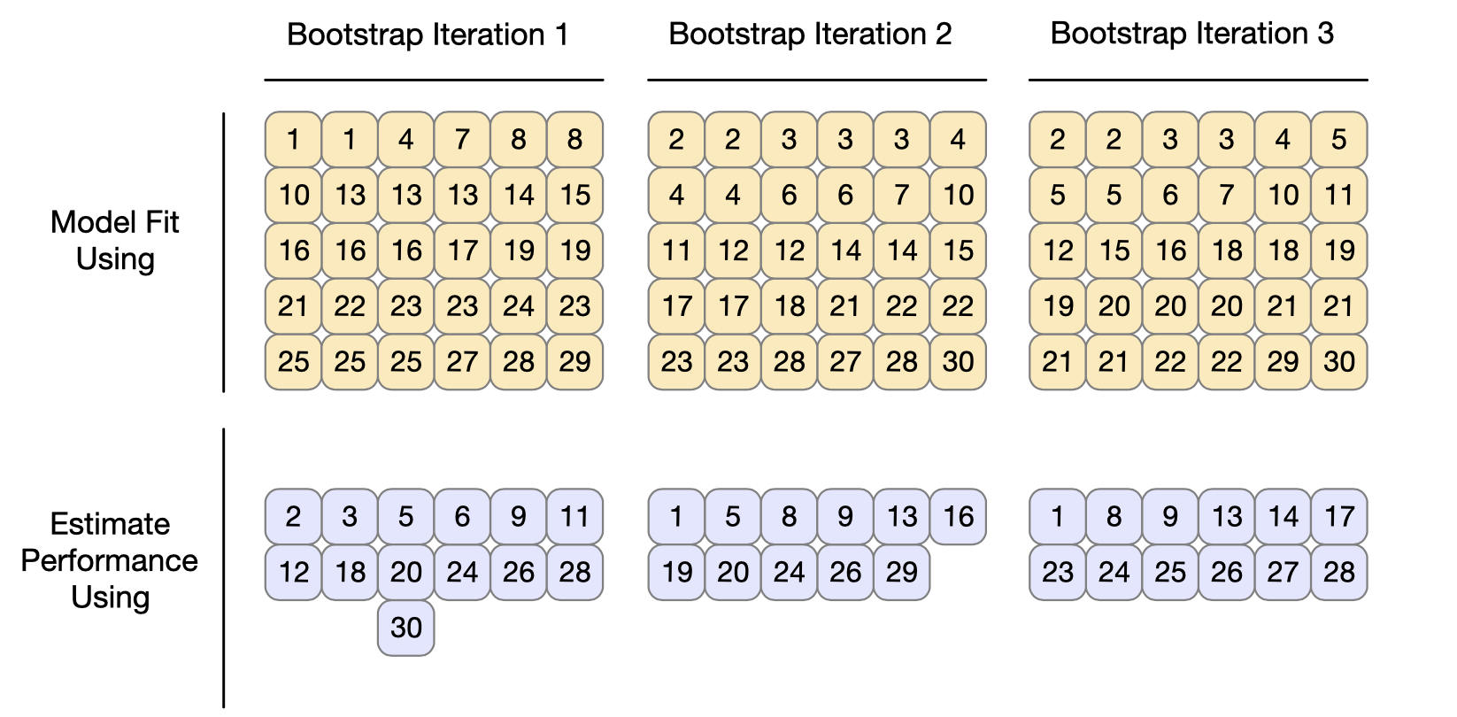
## 1 <split [1756/586]> validation

10.3.3 Boostrapping

Bootstrapping can be used to estimate model performance. It’s good to be aware that while it does produce lower variance compared to other resampling methods, it has “significant pessimistic bias”. It also works differently than other resampling methods. In the diagram below, we can see that the analysis set is always equal to the size of the whole training set, and we can also see that the same points can be selected multiple times. The assessment sets contain the data points that were not previously included in the analysis sets. Furthermore, these assessment sets are not of the same size, as we’re about to see when we call bootstraps().

Operationally, performing bootstrap resampling involves specifying the number of bootstrap samples via the times argument. There is also a strata argument for conducting stratified sampling.

bootstraps(ames_train, times = 5)

## # Bootstrap sampling 
## # A tibble: 5 × 2
##   splits             id        
##   <list>             <chr>     
## 1 <split [2342/830]> Bootstrap1
## 2 <split [2342/867]> Bootstrap2
## 3 <split [2342/856]> Bootstrap3
## 4 <split [2342/849]> Bootstrap4
## 5 <split [2342/888]> Bootstrap5

10.3.4 Rolling forecasting origin resampling

Resampling with time series data needs a special setup as random sampling can ignore important trends such as seasonality. Rolling forecast resampling involves specifying the size of the analysis and assessment sets, and each iteration after the first one skips by a set number as the diagram illustrates below (with a skip of 1 as an example):

This time series resampling is done with rolling_origin. You can specify the number of samples to be used for analysis with initial, the number of samples used for each assessment resample with assess, and cumulative set to true if you want the analysis resample to grow beyong the size specified with initial. Additional arguments include the skip and lag.

rolling_origin(data, initial = 5, assess = 1, cumulative = TRUE, skip = 0, lag = 0)