9.7 Binary Classification Metrics

Note: This code might take several minutes (or longer) to run.

#Cross-fold validation
ames_folds_binary <- vfold_cv(ames, v = 5)

#Create Recipe
ames_recipe_binary <- 
  recipe(formula = under_budget ~ Gr_Liv_Area + Full_Bath + Half_Bath + Lot_Area + Neighborhood + Overall_Cond,
         data = ames)

#Set the model and hyperparameters
ames_spec_binary <- 
    rand_forest(mtry = tune(), trees = tune(), min_n = tune()) %>% 
  set_mode("classification") %>% 
  set_engine("ranger")

#Create workflow
ames_workflow_binary <- 
  workflow() %>%
  add_recipe(ames_recipe_binary) %>%
  add_model(ames_spec_binary)

#Create metric set of all binary metrics
ames_tune_binary <-
  tune_grid(
    ames_workflow_binary,
    metrics =
      metric_set(sens,spec,recall,precision,mcc,j_index,f_meas,accuracy,
                 kap,ppv,npv,bal_accuracy,detection_prevalence),
    resamples = ames_folds_binary,
    grid = grid_regular(
      mtry(range = c(2, 6)),
      min_n(range = c(2, 20)),
      trees(range = c(10,100)),
      levels = 10
    )
  )

#Pick the best model for each metric and pull out the predictions
best_models_binary <- 
  tibble(
    metric_name = c('recall','sens','spec', 'precision','mcc','j_index','f_meas','accuracy',
                    'kap','ppv','npv','bal_accuracy','detection_prevalence')) %>% 
  mutate(metric_best = map(metric_name, ~select_best(ames_tune_binary, .x)),
         wf_best = map(metric_best, ~finalize_workflow(ames_workflow_binary, .x)),
         fit_best = map(wf_best, ~fit(.x, data = ames)),
         df_pred = map(fit_best, ~ames %>% bind_cols(predict(.x, new_data = ames)) %>% select(under_budget, .pred_class))) %>%
  select(-c(wf_best, fit_best)) %>% 
  unnest(cols = c(metric_name, metric_best, df_pred))

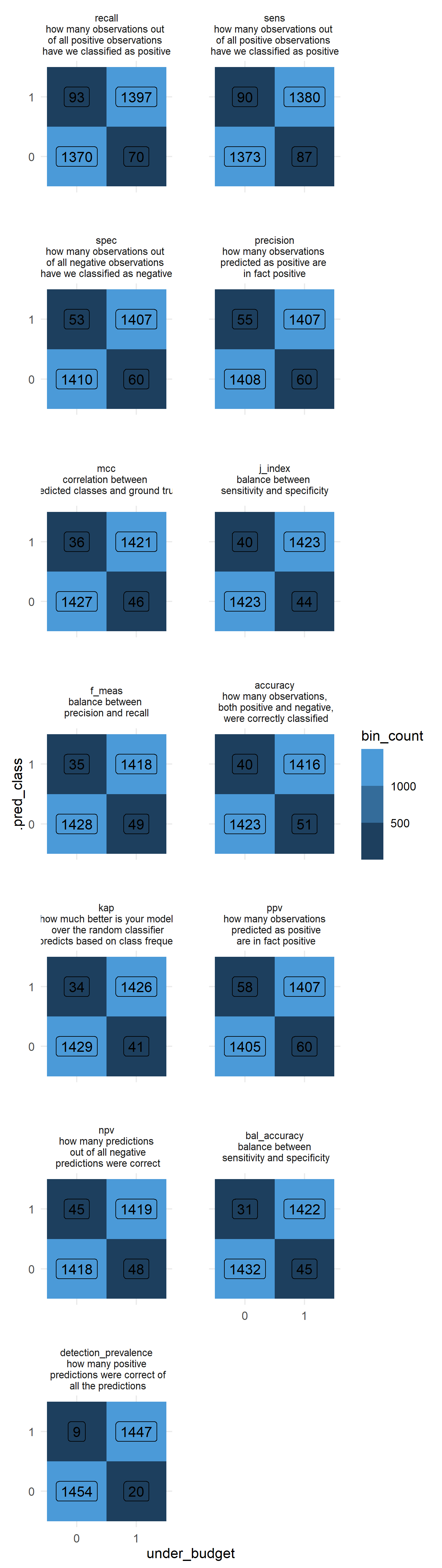
# Plot!
best_models_binary %>%
  mutate(metric_desc = factor(
    metric_name, 
    levels = c('recall','sens','spec', 'precision','mcc','j_index','f_meas','accuracy',
               'kap','ppv','npv','bal_accuracy','detection_prevalence'),
    labels = c('recall\nhow many observations out \nof all positive observations \nhave we classified as positive',
               'sens\nhow many observations out \nof all positive observations \nhave we classified as positive',
               'spec\nhow many observations out \nof all negative observations \nhave we classified as negative', 
               'precision\nhow many observations \npredicted as positive are \nin fact positive',
               'mcc\ncorrelation between \npredicted classes and ground truth',
               'j_index\nbalance between \nsensitivity and specificity',
               'f_meas\nbalance between \nprecision and recall',
               'accuracy\nhow many observations,\n both positive and negative,\n were correctly classified',
               'kap\nhow much better is your model\n over the random classifier\n that predicts based on class frequencies',
               'ppv\nhow many observations\n predicted as positive\n are in fact positive',
               'npv\nhow many predictions\n out of all negative\n predictions were correct',
               'bal_accuracy\nbalance between\n sensitivity and specificity',
               'detection_prevalence\nhow many positive\n predictions were correct of\n all the predictions'))) %>% 
  group_by(metric_desc, under_budget, .pred_class) %>% 
  summarise(bin_count = n()) %>% 
  ungroup() %>% 
  ggplot(aes(x = under_budget, y = .pred_class, fill = bin_count, label = bin_count)) +
  scale_fill_binned() +
  geom_tile() +
  geom_label() +
  coord_fixed() +
  facet_wrap(~metric_desc, ncol = 2) +
  theme_minimal() +
  theme(panel.spacing = unit(2, "lines"),
        strip.text.x = element_text(size = 8))