13.1 Regular and non-regular grids
Let’s consider an example model: an mlp neural network model. The parameters marked for tuning are:
the number of hidden units,
the number of fitting epochs in model training, and
the amount of weight decay penalization.
Using parsnip, the specification for a regression model fit using the nnet package for a multi layer perceptron is:
mlp_spec <-
  mlp(hidden_units = tune(),
      penalty = tune(),
      epochs = tune()) %>%
  set_engine("nnet", trace = 0) %>%
  set_mode("regression")
The argument trace = 0 prevents extra logging of the training process. The parameters() function can extract the set of arguments with unknown values and set their dials objects. extract_parameter_dials() gives the current range of values.
mlp_param <- parameters(mlp_spec)
mlp_param %>% extract_parameter_dials("hidden_units")
## # Hidden Units (quantitative)
## Range: [1, 10]mlp_param %>% extract_parameter_dials("penalty")## Amount of Regularization (quantitative)
## Transformer: log-10 [1e-100, Inf]
## Range (transformed scale): [-10, 0]For
penalty, the random numbers are uniform on the log (base 10) scale. The values in the grid are in their natural units.

mlp_param %>% extract_parameter_dials("epochs")## # Epochs (quantitative)
## Range: [10, 1000]13.1.1 Regular Grids
The dials package contains a set of grid_*() functions that take the parameter object and produce different types of grids.
grid_regular(mlp_param, levels = 2) ## # A tibble: 8 × 3
## hidden_units penalty epochs
## <int> <dbl> <int>
## 1 1 0.0000000001 10
## 2 10 0.0000000001 10
## 3 1 1 10
## 4 10 1 10
## 5 1 0.0000000001 1000
## 6 10 0.0000000001 1000
## 7 1 1 1000
## 8 10 1 1000The levels argument is the number of levels per parameter to create. It can also take a named vector of values:
mlp_param %>%
  grid_regular(levels = c(hidden_units = 3,
                          penalty = 2,
                          epochs = 2))
## # A tibble: 12 × 3
## hidden_units penalty epochs
## <int> <dbl> <int>
## 1 1 0.0000000001 10
## 2 5 0.0000000001 10
## 3 10 0.0000000001 10
## 4 1 1 10
## 5 5 1 10
## 6 10 1 10
## 7 1 0.0000000001 1000
## 8 5 0.0000000001 1000
## 9 10 0.0000000001 1000
## 10 1 1 1000
## 11 5 1 1000
## 12 10 1 1000Regular grids can be computationally expensive to use, especially when there are a large number of tuning parameters. This is true for many models but not all. There are some models whose tuning time decreases with a regular grid. More on this in a moment.
One advantage of a regular grid is that the relationships between the tuning parameters and the model metrics are easily understood. The full factorial nature of designs allows for examination of each parameter separately.
13.1.2 Irregular Grids
Even with small grids, random values can still result in overlaps. Also, the random grid needs to cover the whole parameter space.
Even for a sample of 15 candidate points, this plot shows some overlap between points for our example:
library(ggforce)
set.seed(200)
mlp_param %>%
  # The 'original = FALSE' option keeps penalty in log10 units
  grid_random(size = 15, original = FALSE) %>%
  ggplot(aes(x = .panel_x, y = .panel_y)) +
  geom_point() +
  geom_blank() +
  facet_matrix(vars(hidden_units, penalty, epochs), layer.diag = 2) +
  labs(title = "Random design with 15 candidates")

ggsave(filename = "images/13_grid_random.png")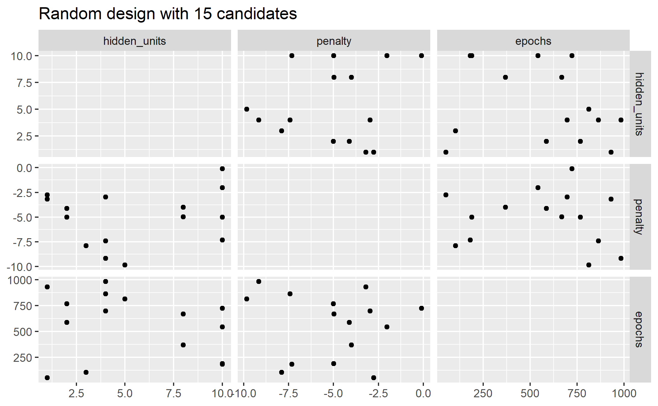
A much better approach is to use designs called
13.1.2.1 Space Filling Designs !!!
They generally find a configuration of points that cover the parameter space with the smallest chance of overlapping. The dials package has:
Latin hypercube
Maximum entropy
As with grid_random(), the primary inputs are the number of parameter combinations and a parameter object.
library(ggforce)
set.seed(200)
mlp_param %>%
  grid_latin_hypercube(size = 15, original = FALSE) %>%
  ggplot(aes(x = .panel_x, y = .panel_y)) +
  geom_point() +
  geom_blank() +
  facet_matrix(vars(hidden_units, penalty, epochs), layer.diag = 2) +
  labs(title = "Latin Hypercube design with 15 candidates")

ggsave("images/13_latin_hypercube.png")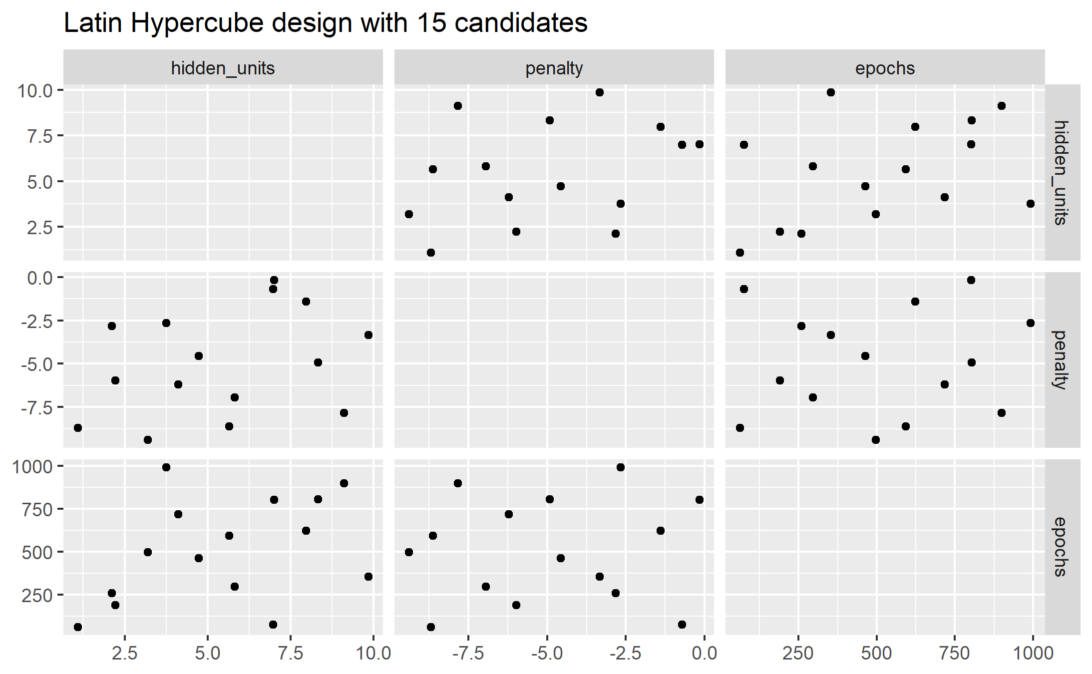
The default design used by tune: maximum entropy design.