21.5 Inference with lower level helpers

Most useful for models not supported by anova, or parsnip, etc or when you want to have more control.

formulas <- list(
  "full" = as.formula(avg_velocity ~ avg_elevation_gain + distance + aid_stations),
  "partial" = as.formula(avg_velocity ~ avg_elevation_gain + distance),
  "minimal" = as.formula(avg_velocity ~ avg_elevation_gain)
)

lm_spec <- linear_reg() %>% set_engine("lm")

AICs <- map(formulas, function(formula) {
  lm_spec %>%
    fit(formula, data = race_top_results) %>%
    extract_fit_engine() %>%
    AIC()
})
AICs

## $full
## [1] 3123.333
## 
## $partial
## [1] 3122.497
## 
## $minimal
## [1] 3148.007

How to determine whether these differences are significant? One possible solution is bootstrapping which can also be used when there are no nice theoretical properties.

velocity_model_summaries <- race_top_results %>%
  bootstraps(times = 1000, apparent = TRUE) %>%
  mutate(
    full_aic = map_dbl(splits, ~ fit(lm_spec, formulas[["full"]], data = analysis(.x)) %>% extract_fit_engine() %>% AIC()),
    partial_aic = map_dbl(splits, ~ fit(lm_spec, formulas[["partial"]], data = analysis(.x)) %>% extract_fit_engine() %>% AIC()),
    minimal_aic = map_dbl(splits, ~ fit(lm_spec, formulas[["minimal"]], data = analysis(.x)) %>% extract_fit_engine() %>% AIC())
  ) %>% 
  select(full_aic, partial_aic, minimal_aic)

velocity_model_summaries %>%
  pivot_longer(c(full_aic, partial_aic, minimal_aic)) %>%
  ggplot(aes(x = name, y = value)) +
  geom_boxplot()

velocity_model_summaries %>%
  summarize(
    full_vs_partial = mean(full_aic < partial_aic),
    partial_vs_minimal = mean(partial_aic < minimal_aic)
  )

## # A tibble: 1 × 2
##   full_vs_partial partial_vs_minimal
##             <dbl>              <dbl>
## 1           0.377              0.916

velocity_model_summaries %>%
  unnest(full_coeffs) %>%
  ggplot(aes(x = estimate)) +
  geom_histogram(bins = 5) +
  facet_wrap(~term, scales = "free_x") +
  geom_vline(xintercept = 0, col = "green")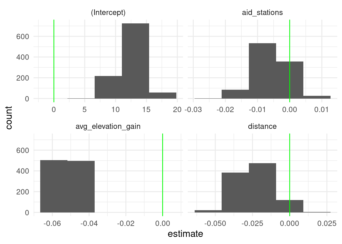

Small reps used for speed

race_top_results %>%
  bootstraps(times = 20) %>%
  mutate(
    full_coeffs = map(splits, ~ fit(lm_spec, formulas[["full"]], data = analysis(.x)) %>% tidy())
  ) %>% 
  int_pctl(full_coeffs)

## # A tibble: 4 × 6
##   term                .lower .estimate   .upper .alpha .method   
##   <chr>                <dbl>     <dbl>    <dbl>  <dbl> <chr>     
## 1 (Intercept)         9.89    12.9     15.5       0.05 percentile
## 2 aid_stations       -0.0139  -0.00512  0.00607   0.05 percentile
## 3 avg_elevation_gain -0.0554  -0.0515  -0.0465    0.05 percentile
## 4 distance           -0.0430  -0.0261  -0.00765   0.05 percentile

The key components are bootstraps() and mutate + map which give you quite a bit of flexibility to compute many statistics.