13.2 Evaluating the grid

“To choose the best tuning parameter combination, each candidate set is assessed using data on cross validation slices that were not used to train that model.”
The user selects the most appropriate set. It might make sense to choose the empirically best parameter combination or bias the choice towards other aspects like simplicity.
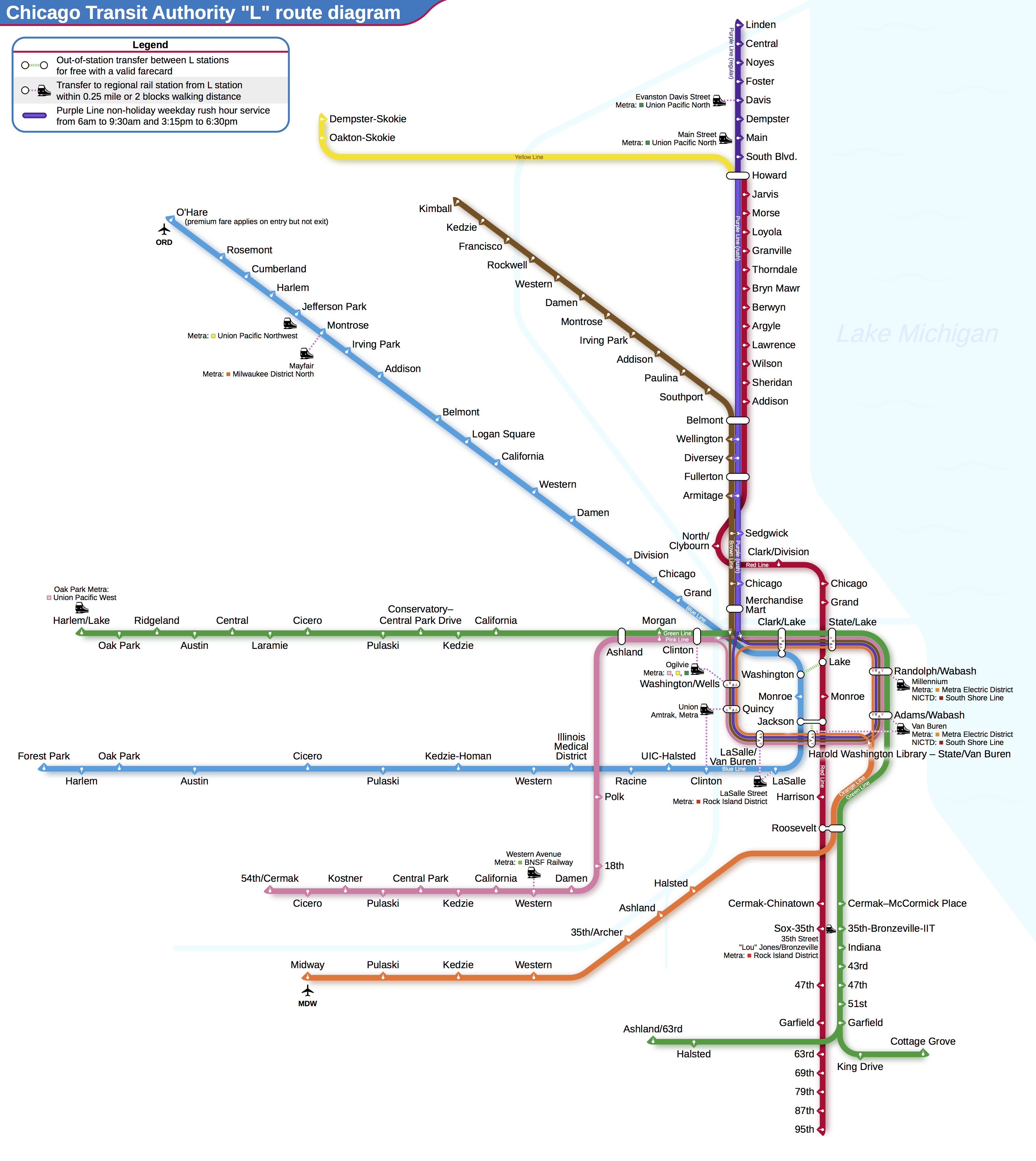
We will use the Chicago CTA data for modeling the number of people (in thousands) who enter the Clark and Lake L station, as ridership.
The date column corresponds to the current date.
The columns with station names (Austin through California) are 14 day lag variables. There are also columns related to weather and sports team schedules.
data(Chicago) # from the modeldata package

# also live data via RSocrata and Chicago portal

glimpse(Chicago, width = 5)
## Rows: 5,698
## Columns: 50
## $ ridership <dbl> …
## $ Austin <dbl> …
## $ Quincy_Wells <dbl> …
## $ Belmont <dbl> …
## $ Archer_35th <dbl> …
## $ Oak_Park <dbl> …
## $ Western <dbl> …
## $ Clark_Lake <dbl> …
## $ Clinton <dbl> …
## $ Merchandise_Mart <dbl> …
## $ Irving_Park <dbl> …
## $ Washington_Wells <dbl> …
## $ Harlem <dbl> …
## $ Monroe <dbl> …
## $ Polk <dbl> …
## $ Ashland <dbl> …
## $ Kedzie <dbl> …
## $ Addison <dbl> …
## $ Jefferson_Park <dbl> …
## $ Montrose <dbl> …
## $ California <dbl> …
## $ temp_min <dbl> …
## $ temp <dbl> …
## $ temp_max <dbl> …
## $ temp_change <dbl> …
## $ dew <dbl> …
## $ humidity <dbl> …
## $ pressure <dbl> …
## $ pressure_change <dbl> …
## $ wind <dbl> …
## $ wind_max <dbl> …
## $ gust <dbl> …
## $ gust_max <dbl> …
## $ percip <dbl> …
## $ percip_max <dbl> …
## $ weather_rain <dbl> …
## $ weather_snow <dbl> …
## $ weather_cloud <dbl> …
## $ weather_storm <dbl> …
## $ Blackhawks_Away <dbl> …
## $ Blackhawks_Home <dbl> …
## $ Bulls_Away <dbl> …
## $ Bulls_Home <dbl> …
## $ Bears_Away <dbl> …
## $ Bears_Home <dbl> …
## $ WhiteSox_Away <dbl> …
## $ WhiteSox_Home <dbl> …
## $ Cubs_Away <dbl> …
## $ Cubs_Home <dbl> …
## $ date <date> …Ridership is the dependent variable. Sorted by oldest to newest date, it matches exactly the Clark_Lake lagged by 14 days.
Chicago$ridership[25:27]## [1] 15.685 15.376 2.445Chicago$Clark_Lake[39:41]## [1] 15.685 15.376 2.445Ridership is in thousands per day and ranges from 600 to 26,058
summary(Chicago$ridership)## Min. 1st Qu. Median Mean 3rd Qu. Max.
## 0.601 6.173 15.902 13.619 18.931 26.058Cross validation folds here are taken on a sliding window
set.seed(33)
split <- rsample::initial_time_split(Chicago)
Chicago_train <- training(split)
Chicago_test <- testing(split)

Chicago_folds <- sliding_period(
  Chicago_train,
  index = date,
  period = "year",
  lookback = 3,
  assess_stop = 1
)
Training and validation data range
range(Chicago_train$date)## [1] "2001-01-22" "2012-10-03"Testing data range
range(Chicago_test$date)## [1] "2012-10-04" "2016-08-28"ggplot(Chicago_folds %>% tidy(),
aes(x = Resample, y = Row, fill = Data)) +
geom_tile() 
Because of the high degree of correlation between predictors, it makes sense to use PCA feature extraction.
While the resulting PCA components are technically on the same scale, the lower-rank components tend to have a wider range than the higher-rank components. For this reason, we normalize again to coerce the predictors to have the same mean and variance.
The resulting recipe:
mlp_rec <-
  recipe(ridership ~ .,
         data = Chicago_train) %>%
  step_date(date,
            features = c("dow", "month"),
            ordinal = FALSE) %>%
  step_rm(date) %>%
  step_normalize(all_numeric(),
                 -ridership) %>% # remove the dependent
  step_pca(all_numeric(),
           -ridership,
           num_comp = tune()) %>%
  step_normalize(all_numeric(),
                 -ridership) # remove the dependent

mlp_wflow <-
  workflow() %>%
  add_model(mlp_spec) %>%
  add_recipe(mlp_rec)
In
step_pca(), using zero PCA components is a shortcut to skip the feature extraction. In this way, the original predictors can be directly compared to the results that include PCA components.
Let’s create a parameter object to adjust a few of the default ranges.
mlp_param <-
  mlp_wflow %>%
  parameters() %>%
  update(
    epochs = epochs(c(50, 200)),
    num_comp = num_comp(c(0, 20))
  )

rmse_mape_rsq_iic <- metric_set(rmse,
                                mape,
                                rsq,
                                iic)
tune_grid() is the primary function for conducting grid search. It resembles fit_resamples() from prior chapters, but adds
grid: An integer or data frame. When an integer is used, the function creates a space-filling design. If specific parameter combinations exist, the grid parameter is used to pass them to the function.
param_info: An optional argument for defining the parameter ranges, when grid is an integer.
set.seed(99)
mlp_reg_tune <-
  mlp_wflow %>%
  tune_grid(
    Chicago_folds,
    grid = mlp_param %>% grid_regular(levels = 3),
    metrics = rmse_mape_rsq_iic
  )

write_rds(mlp_reg_tune,
          file = "data/13-Chicago-mlp_reg_tune.rds",
          compress = "gz")
There are high-level convenience functions to understand the results. First, the autoplot() method for regular grids shows the performance profiles across tuning parameters:
autoplot(mlp_reg_tune) + theme(legend.position = "top")

ggsave("images/13_mlp_reg_tune_autoplot.png",
       width = 12)
The best model, per the index of ideality of correlation (iic), on the validation folds
More study might be warranted to dial in the resolution of the penalty and number of pca components.
To evaluate the same range using (the tune grid default) maximum entropy design with 20 candidate values:
set.seed(99)
mlp_sfd_tune <-
  mlp_wflow %>%
  tune_grid(
    Chicago_folds,
    grid = 20,
    # Pass in the parameter object to use the appropriate range:
    param_info = mlp_param,
    metrics = rmse_mape_rsq_iic
  )

write_rds(mlp_sfd_tune,
          file = "data/13-Chicago-mlp_max_entropy.rds",
compress = "gz")autoplot(mlp_sfd_tune)
ggsave("images/13_mlp_max_entropy_plot.png")
Care should be taken when examining this plot; since a regular grid is not used, the values of the other tuning parameters can affect each panel.
show_best(mlp_sfd_tune, metric = "iic") %>% select(-.estimator) hidden_units penalty epochs num_comp .metric mean n std_err .config
<int> <dbl> <int> <int> <chr> <dbl> <int> <dbl> <chr>
1 9 7.80e- 3 158 14 iic 0.790 8 0.0439 Preprocessor~
2 4 7.01e- 9 173 18 iic 0.779 8 0.0375 Preprocessor~
3 10 2.96e- 4 155 19 iic 0.777 8 0.0293 Preprocessor~
4 8 2.96e- 6 69 19 iic 0.760 8 0.0355 Preprocessor~
5 5 8.76e-10 199 9 iic 0.756 8 0.0377 Preprocessor~It often makes sense to choose a slightly suboptimal parameter combination that is associated with a simpler model. For this model, simplicity corresponds to larger penalty values and/or fewer hidden units.