8.4 HOW DATA ARE USED BY THE RECIPE
8.4.1 EXAMPLES OF RECIPE STEPS:
- ENCODING QUALITATIVE DATA IN A NUMERIC FORMAT
step_unknown() change missing values to a dedicated factor level
step_novel() a new factor level may be encountered in future data
step_other() to analyze the frequencies of the factor levels
the bottom 1% of the neighborhoods will be lumped into a new level called “other”
step_other(Neighborhood, threshold = 0.01)- step_dummy() for converting a factor predictor to a numeric format (one_hot argument to include the reference variable)
simple_ames <-
  recipe(Sale_Price ~ Neighborhood + Gr_Liv_Area + Year_Built + Bldg_Type,
         data = ames_train) %>%
  step_log(Gr_Liv_Area, base = 10) %>%
  step_other(Neighborhood, threshold = 0.01) %>%
step_dummy(all_nominal_predictors())- INTERACTION TERMS
- step_interact(~ interaction terms)
one predictor has an effect on the outcome that is contingent on one or more other predictors
Numerically, an interaction term between predictors is encoded as their product.
ggplot(ames_train, aes(x = Gr_Liv_Area, y = Sale_Price)) +
  geom_point(alpha = .2) +
  facet_wrap(~ Bldg_Type) +
  geom_smooth(method = lm, formula = y ~ x, se = FALSE, color = "lightblue") +
  scale_x_log10() +
  scale_y_log10() +
  labs(x = "Gross Living Area", y = "Sale Price (USD)")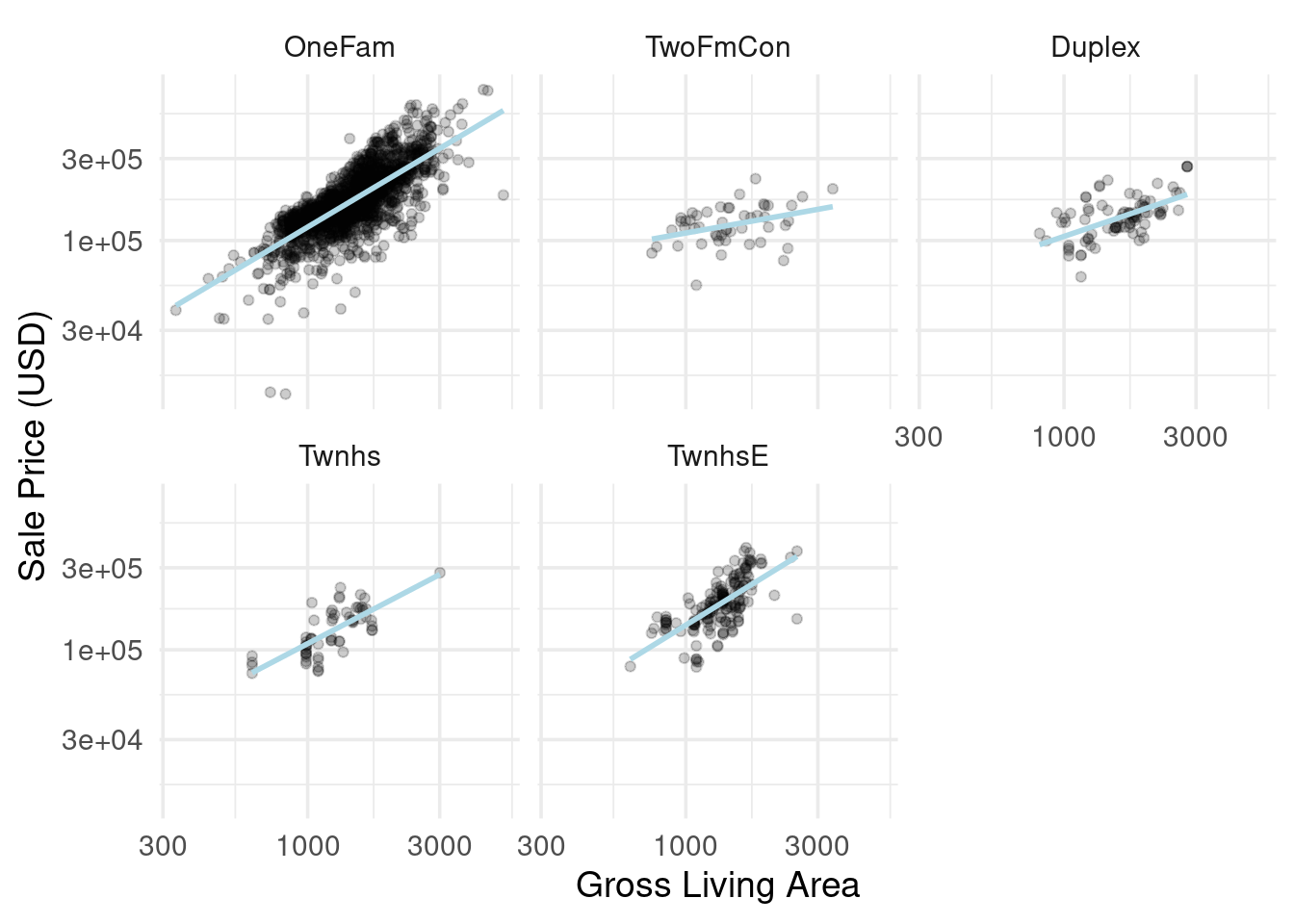
Sale_Price ~ Neighborhood + log10(Gr_Liv_Area) + Bldg_Type + log10(Gr_Liv_Area):Bldg_Typeor
Sale_Price ~ Neighborhood + log10(Gr_Liv_Area) * Bldg_Type simple_ames <-
recipe(Sale_Price ~ Neighborhood + Gr_Liv_Area + Year_Built + Bldg_Type,
data = ames_train) %>%
step_log(Gr_Liv_Area, base = 10) %>%
step_other(Neighborhood, threshold = 0.01) %>%
step_dummy(all_nominal_predictors()) %>%
# Gr_Liv_Area is on the log scale from a previous step
step_interact( ~ Gr_Liv_Area:starts_with("Bldg_Type_") )Additional interactions can be specified in this formula by separating them by +
- SPLINE FUNCTIONS
- step_ns() for non-linear relationships
Splines replace the existing numeric predictor with a set of columns that allow a model to emulate a flexible, non-linear relationship
library(patchwork)
library(splines)

plot_smoother <- function(deg_free) {
  ggplot(ames_train, aes(x = Latitude, y = 10^Sale_Price)) +
    geom_point(alpha = .2) +
    scale_y_log10() +
    geom_smooth(
      method = lm,
      formula = y ~ ns(x, df = deg_free),
      color = "lightblue",
      se = FALSE
    ) +
    labs(title = paste(deg_free, "Spline Terms"),
         y = "Sale Price (USD)")
}

( plot_smoother(2) + plot_smoother(5) ) / ( plot_smoother(20) + plot_smoother(100) )
recipe(Sale_Price ~ Neighborhood + Gr_Liv_Area + Year_Built + Bldg_Type + Latitude,
         data = ames_train) %>%
  step_log(Gr_Liv_Area, base = 10) %>%
  step_other(Neighborhood, threshold = 0.01) %>%
  step_dummy(all_nominal_predictors()) %>%
  step_interact( ~ Gr_Liv_Area:starts_with("Bldg_Type_") ) %>%
step_ns(Latitude, deg_free = 20)- FEATURE EXTRACTION
step_normalize() center and scale each column
step_pca() principal component analysis, it extracts as much of the original information in the predictor set as possible using a smaller number of features,reducing the correlation between predictors.
step_pca(matches(“(SF$)|(Gr_Liv)”))
step_ica() independent component analysis
step_umap() uniform manifold approximation and projection
- ROW SAMPLING STEPS
Downsampling ({themis} package)
step_downsample(outcome_column_name)
Upsampling
Hybrid methods
step_filter(), step_sample(), step_slice(), and step_arrange() …
- GENERAL TRANSFORMATIONS
- step_mutate()
- NATURAL LANGUAGE PROCESSING
can apply natural language processing methods to the data