21.3 {infer} for simple, high level hypothesis testing

• specify relationship and optionally hypothesis
• calculate statistics from simulation or based on theoretical distributions
• many common tests are supported for continuous and discreet variables as well

21.3.1 p value for idependence based on simulation with permutation

observed <- race_top_results %>%
  specify(avg_velocity ~ avg_elevation_gain) %>%
  calculate(stat = "correlation")

observed

## Response: avg_velocity (numeric)
## Explanatory: avg_elevation_gain (numeric)
## # A tibble: 1 × 1
##     stat
##    <dbl>
## 1 -0.561

permuted <- race_top_results %>%
  specify(avg_velocity ~ avg_elevation_gain) %>%
  hypothesise(null = "independence") %>%
  generate(reps = 1000, type = "permute") %>%
  calculate(stat = "correlation")

permuted

## Response: avg_velocity (numeric)
## Explanatory: avg_elevation_gain (numeric)
## Null Hypothesis: independence
## # A tibble: 1,000 × 2
##    replicate     stat
##        <int>    <dbl>
##  1         1 -0.0108 
##  2         2  0.0193 
##  3         3 -0.00134
##  4         4 -0.0564 
##  5         5 -0.0386 
##  6         6 -0.0142 
##  7         7 -0.0359 
##  8         8 -0.0313 
##  9         9 -0.00306
## 10        10 -0.0488 
## # ℹ 990 more rows

permuted %>%
  visualize() +
  shade_p_value(observed, direction = "two_sided")

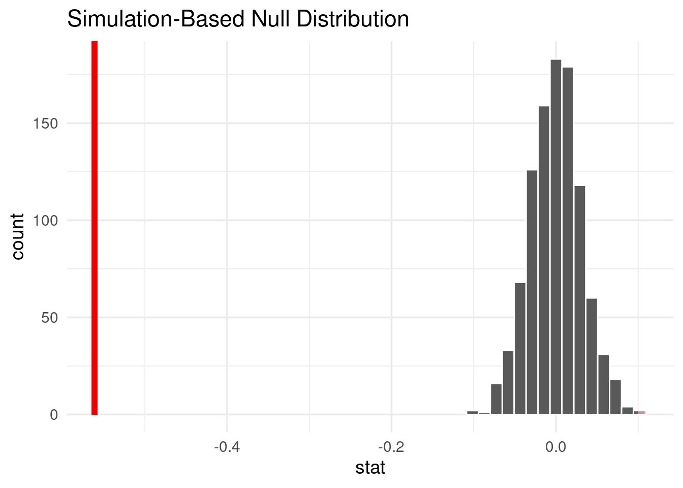
get_p_value(permuted, observed, direction = "two_sided")

## # A tibble: 1 × 1
##   p_value
##     <dbl>
## 1       0

21.3.2 Confidence interval for correlation based on simulation with bootstrapping

bootstrapped <- race_top_results %>%
  specify(avg_velocity ~ avg_elevation_gain) %>%
  generate(reps = 1000, type = "bootstrap") %>%
  calculate(stat = "correlation")

bootstrapped %>%
  visualize() +
  shade_confidence_interval(get_confidence_interval(bootstrapped))

21.3.3 Use theory instead of simulation

observed_t <- race_top_results %>%
  specify(response = avg_velocity) %>%
  hypothesise(null = "point", mu = 7) %>%
  calculate(stat = "t")

race_top_results %>%
  specify(response = avg_velocity) %>%
  assume("t") %>%
  visualize() +
  shade_p_value(observed_t, direction = "two_sided")

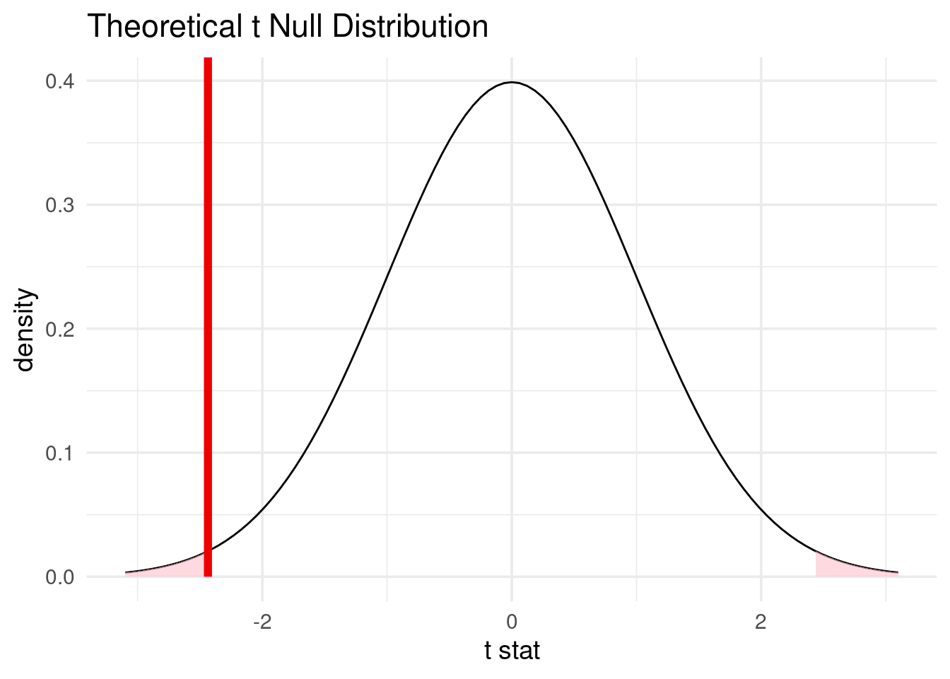
race_top_results %>%
  specify(response = avg_velocity) %>%
  assume("t") %>%
  get_p_value(observed_t, "two_sided")

## # A tibble: 1 × 1
##   p_value
##     <dbl>
## 1  0.0150

21.3.4 Linear models with multiple explanatory variables

my_formula <- as.formula(avg_velocity ~ aid_stations + participants)

observed_fit <- race_top_results %>%
  specify(my_formula) %>%
  fit()

observed_fit

## # A tibble: 3 × 2
##   term          estimate
##   <chr>            <dbl>
## 1 intercept     6.93    
## 2 aid_stations -0.0127  
## 3 participants  0.000432

permuted_fits <- race_top_results %>%
  specify(my_formula) %>%
  hypothesise(null = "independence") %>%
  generate(reps = 1000, type = "permute", variables = c(aid_stations, participants)) %>%
  fit()

bootstrapped_fits <- race_top_results %>%
  specify(my_formula) %>%
  generate(reps = 2000, type = "bootstrap") %>%
  fit()

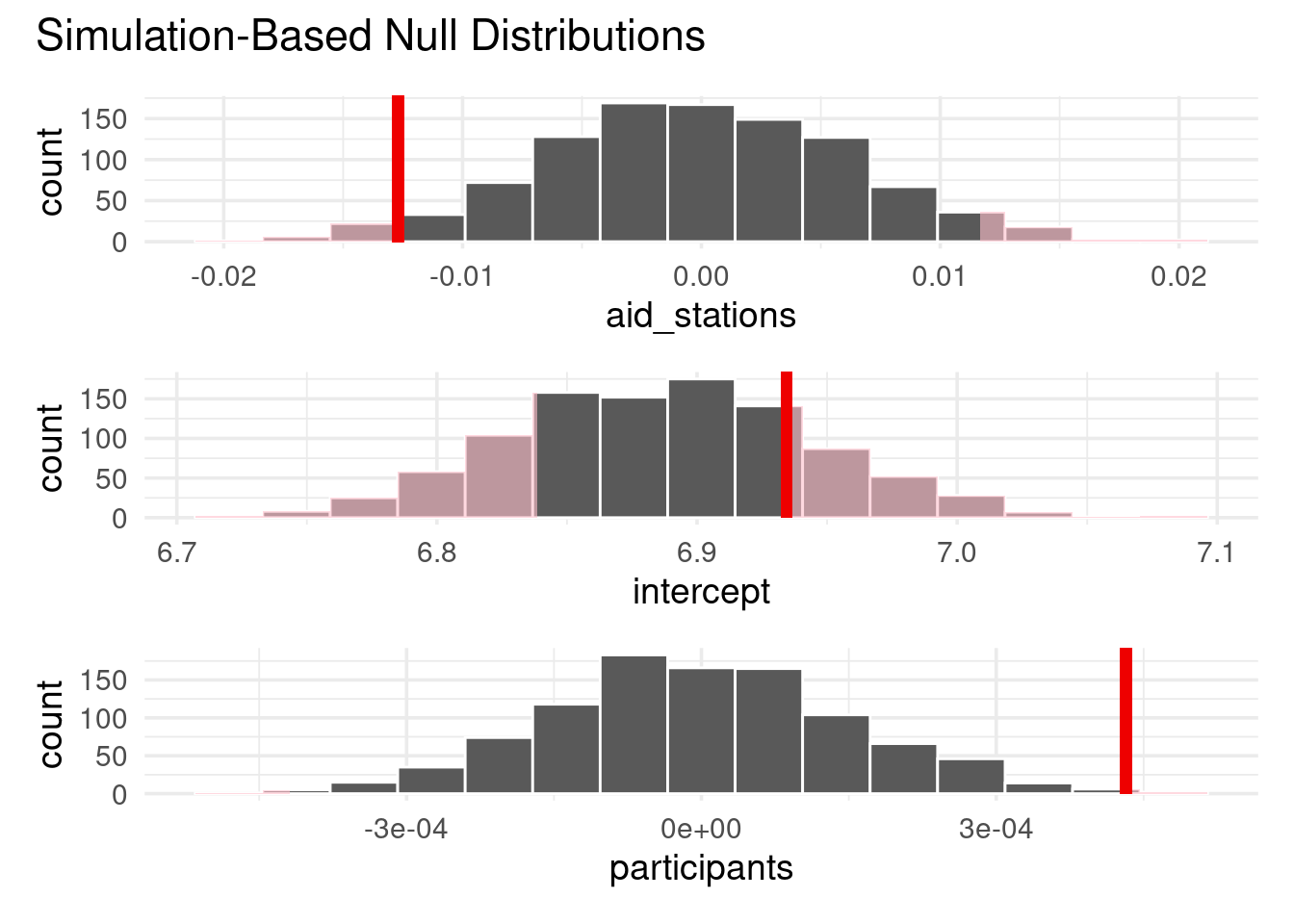
permuted_fits %>% get_p_value(observed_fit, "two_sided")

## # A tibble: 3 × 2
##   term         p_value
##   <chr>          <dbl>
## 1 aid_stations   0.058
## 2 intercept      0.412
## 3 participants   0.004

visualize(permuted_fits) +
  shade_p_value(observed_fit, "two_sided")

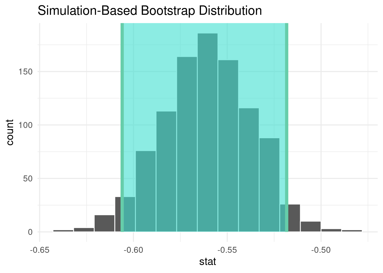
bootstrapped_fits %>%
  get_confidence_interval(type = "percentile", point_estimate = observed_fit)

## # A tibble: 3 × 3
##   term          lower_ci upper_ci
##   <chr>            <dbl>    <dbl>
## 1 aid_stations -0.0278   0.00223 
## 2 intercept     6.80     7.07    
## 3 participants  0.000123 0.000890