14.2 Bayesian Optimization
Bayesian optimization is one of the techniques that can be used to iteratively search for new tuning parameter values.
Bayesian optimization consists of the following steps:
create a model predicting new tuning parameter values based on the previously generated resampling results
resampling of the new tuning parameter values
create another model that recommends additional tuning parameter values based on the resampling results of the previous step
This process can occur:
for a predetermined number of iterations, or
until there is no improvement in the results
Let’s go over the most commonly used technique for Bayesian optimization, called the Gaussian process model.
14.2.1 Gaussian process model, at a high level
In plain terms, Gaussian processes (GP) models allow us to make predictions about our data by incorporating prior knowledge and fitting a function to the data. With a given set of training points, there are potentially an infinite number of functions. GP shine by giving each of these functions a probability. This generates a probability distribution, which can harnessed.
14.2.1.1 How is it used for tuning?
As the name suggests, the Gaussian distribution is central to GP models. We’re interested in the multivariate case of this distribution, where each random variable is distributed normally and their joint distribution is also Gaussian.
This collection of random variables in the context of our example is the collection of performance metrics for the tuning parameter candidate values. The 25 random variables making up the grid for our SVM model is assumed to be distributed as multivariate Gaussian.
For the GP model:
the inputs (i.e. predictors) are the tuning parameters,
costandrbf_sigmathe outcome is the performance metric, ROC AUC
the outputs are predicted mean and variance (of ROC AUC) for the new candidate tuning parameters
- note: the predicted variance is mostly driven by how far it is from existing data
A candidate is selected
Performance estimate are calculated for all existing results
This process is iterative, and keeps repeating until number of iterations is exhausted or no improvement occurs.
See Max and Julia’s notes for an in-depth appreciation of the mathematical implications of GP, along with this excellent interactive blog post by researchers at the University of Konstanz. The elegant properties of GP allow us to:
compute new performance statistics because we obtain a full probability model which reflects the entire distribution of the outcome
represent highly non-linear relationships between model performance and the tuning parameters
While it’s a powerful technique that can yield good results, it can be complex to set up. The two main considerations are:
how to set up the model
how to pick the parameter values suggested by the model
resources, as it can be computationally expensive
Point 2 is further explored in the next section.
14.2.1.2 Acquisition functions
As we saw previously, GP model generates predicted mean and variance for candidate combinations of parameter values. The next step is picking the parameter combination that could give us the best results. This picking process can be tricky, as there is a trade-off between the predicted mean and variance for new candidates. This trade-off is similar to another, the exploration-exploitation trade-off:
Exploration: selection is towards “relatively unexplored” areas i.e. where there are fewer (or no) candidate models. This results in candidates having relatively higher variance, as they are “further” from existing data.
Exploitation: selection is based on the best mean prediction. This results in candidates having relatively lower variance, as it focuses on existing data.
The following is an example consisting of 1 tuning parameter (0,1) where the performance metric is r-squared. The points correspond to the observed candidate values for the tuning parameter. The shaded regions represent the mean +/- 1 standard error.
From an exploitation standpoint, one might select a parameter value right next to the observed point - i.e. near left vertical line - as it has the best r-squared.
From an exploration standpoint, one might consider the parameter value with the largest confidence interval - i.e. near right vertical line - since it would push our selection towards a region with no observed result. This is known as the confidence bound approach.
Max and Julia note that the latter approach is not often used.

This is where acquisition functions come in, as they can help us in this process of picking a suitable parameter value. The most commonly used one is expected improvement. Let’s illustrate how it works by bringing back the two candidate parameter values we were considering, 0.1 and 0.25:

We can see that the distribution for 0.1 is much narrower (red line), and has the best r-squared (vertical line). So, 0.1 is our current best on average; however, we can see that for parameter value 0.25 there is higher variance and more overall probability area above the current best. What does this mean for our expected improvement acquisition function?
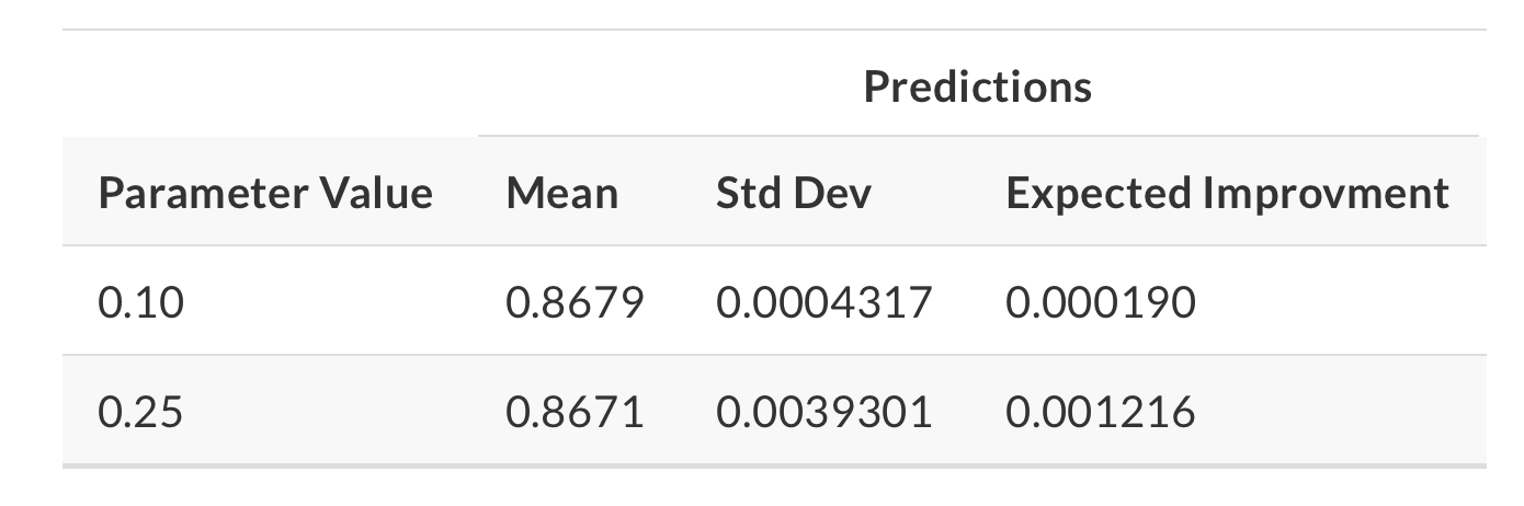
We can see that the expected improvement is significantly higher for parameter value 0.25!
14.2.1.3 The tune_bayes() function
The tune_bayes() function sets up Bayesian optimization iterative search. It’s similar to tune_grid() but with additional arguments. You can specify the maximum number of search iterations, the acquisition function to be used, and whether to stop the search if no improvement is detected. See Max and Julia for details and additional arguments.
Let’s keep going with our SVM model. We can use the earlier SVM results as the initial substrate. Once again, we’re trying to maximize ROC AUC.
ctrl <- control_bayes(verbose = TRUE) # can also add more arguments, like no_improve
set.seed(420)
svm_bo <-
svm_wflow %>%
tune_bayes(
resamples = penguins_folds,
metrics = roc_res,
initial = svm_initial, # tune_grid object produced earlier
param_info = svm_param, # specified earlier too, with our new bounds for rbf_sigma
iter = 25, # maximum number of search iterations
control = ctrl
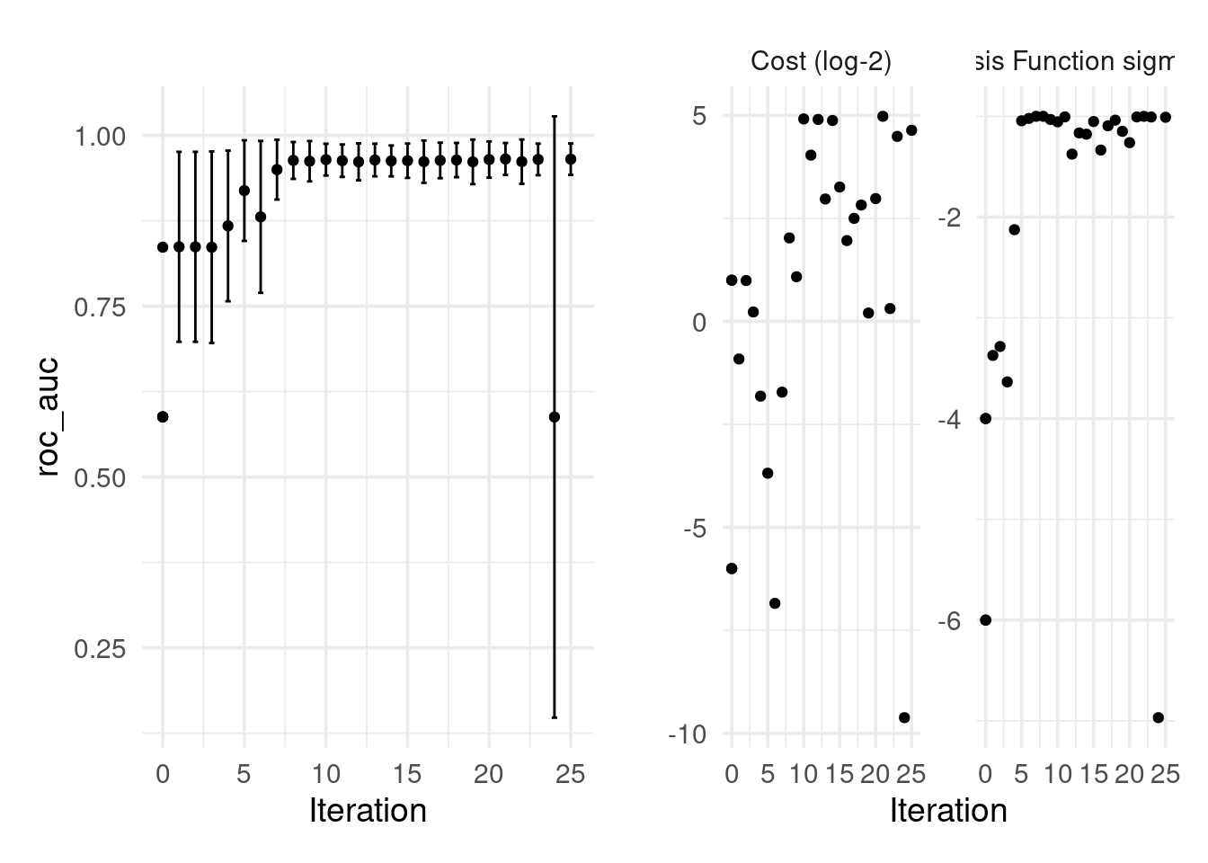
)Looks like the improvements occurred at iterations 8, 11, 13, 12 and 10. We can pull the best result(s) like so:
show_best(svm_bo) # same call as with grid search## # A tibble: 5 × 9
## cost rbf_sigma .metric .estimator mean n std_err .config .iter
## <dbl> <dbl> <chr> <chr> <dbl> <int> <dbl> <chr> <int>
## 1 31.5 0.0986 roc_auc binary 0.965 5 0.00909 Iter21 21
## 2 24.9 0.0979 roc_auc binary 0.965 5 0.00896 Iter25 25
## 3 22.5 0.0984 roc_auc binary 0.965 5 0.00900 Iter23 23
## 4 7.89 0.0548 roc_auc binary 0.965 5 0.0103 Iter20 20
## 5 30.2 0.0881 roc_auc binary 0.964 5 0.00905 Iter10 10p1 <- autoplot(svm_bo, type = "performance")
p2 <- autoplot(svm_bo, type = "parameters")
p1 + p2