5.3 Class imbalance

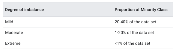
In many instances, random splitting is not suitable. This includes datasets that contain class imbalance, meaning one class is dominated by another. Class imbalance is important to detect and take into consideration in data splitting. Performing random splitting on a dataset with severe class imbalance may cause the model to perform badly at validation. You want to avoid allocating the minority class disproportionately into the training or test set. The point is to have the same distribution across the training and test sets. Class imbalance can occur in differing degrees:

Splitting methods suited for datasets containing class imbalance should be considered. Let’s consider a #Tidytuesday dataset on Himalayan expedition members, which Julia Silge recently explored here using {tidymodels}.

library(tidyverse)
library(skimr)
members <- read_csv("https://raw.githubusercontent.com/rfordatascience/tidytuesday/master/data/2020/2020-09-22/members.csv") 

skim(members)

Table 5.1: Data summary

Name	members
Number of rows	76519
Number of columns	21
_______________________
Column type frequency:
character	10
logical	6
numeric	5
________________________
Group variables	None

Variable type: character

skim_variable	n_missing	complete_rate	min	max	empty	n_unique	whitespace
expedition_id	0	1.00	9	9	0	10350	0
member_id	0	1.00	12	12	0	76518	0
peak_id	0	1.00	4	4	0	391	0
peak_name	15	1.00	4	25	0	390	0
season	0	1.00	6	7	0	5	0
sex	2	1.00	1	1	0	2	0
citizenship	10	1.00	2	23	0	212	0
expedition_role	21	1.00	4	25	0	524	0
death_cause	75413	0.01	3	27	0	12	0
injury_type	74807	0.02	3	27	0	11	0

Variable type: logical

skim_variable	n_missing	complete_rate	mean	count
hired	0	1	0.21	FAL: 60788, TRU: 15731
success	0	1	0.38	FAL: 47320, TRU: 29199
solo	0	1	0.00	FAL: 76398, TRU: 121
oxygen_used	0	1	0.24	FAL: 58286, TRU: 18233
died	0	1	0.01	FAL: 75413, TRU: 1106
injured	0	1	0.02	FAL: 74806, TRU: 1713

Variable type: numeric

skim_variable	n_missing	complete_rate	mean	sd	p0	p25	p50	p75	p100	hist
year	0	1.00	2000.36	14.78	1905	1991	2004	2012	2019	▁▁▁▃▇
age	3497	0.95	37.33	10.40	7	29	36	44	85	▁▇▅▁▁
highpoint_metres	21833	0.71	7470.68	1040.06	3800	6700	7400	8400	8850	▁▁▆▃▇
death_height_metres	75451	0.01	6592.85	1308.19	400	5800	6600	7550	8830	▁▁▂▇▆
injury_height_metres	75510	0.01	7049.91	1214.24	400	6200	7100	8000	8880	▁▁▂▇▇

Let’s say we were interested in predicting the likelihood of survival or death for an expedition member. It would be a good idea to check for class imbalance:

library(janitor)

members %>% 
  tabyl(died) %>% 
  adorn_totals("row")

##   died     n    percent
##  FALSE 75413 0.98554607
##   TRUE  1106 0.01445393
##  Total 76519 1.00000000

We can see that nearly 99% of people survive their expedition. This dataset would be ripe for a sampling technique adept at handling such extreme class imbalance. This technique is called stratified sampling, in which “the training/test split is conducted separately within each class and then these subsamples are combined into the overall training and test set”. Operationally, this is done by using the strata argument inside initial_split():

set.seed(123)
members_split <- initial_split(members, prop = 0.80, strata = died)
members_train <- training(members_split)
members_test <- testing(members_split)

5.3.1 Stratified sampling simulation

With simulation we can see the effect of stratification: we expect that the expected value does not change with stratification but the variance is lower.

simulate_stratified_sampling <- function(prop_in_dataset, n_resample = 50,
                                         n_rows = 1000, seed = 45678) {
  set.seed(seed)
  
  data_to_split <- tibble(died = c(
    rep(1, floor(n_rows * prop_in_dataset)),
    rep(0, floor(n_rows * (1 - prop_in_dataset)))
  ))
  
  samples <- map_dfr(seq_len(n_resample), ~{
    initial_split(data_to_split) %>% 
      testing() %>% 
      summarize(died_pct = mean(died))
  }) 
  
  stratified_samples <- map_dfr(seq_len(n_resample), ~{
    initial_split(data_to_split, strata = died) %>% 
      testing() %>% 
      summarize(died_pct = mean(died))
  }) 
  
  rbind(
    samples %>% mutate(stratified = FALSE),
    stratified_samples %>% mutate(stratified = TRUE)
  ) %>% 
    group_by(stratified) %>% 
    summarize(mean = mean(died_pct), var = var(died_pct))
}

rsample does not stratify if class imbalance is more extreme than 10%

simulate_stratified_sampling(0.09)

## # A tibble: 2 × 3
##   stratified   mean      var
##   <lgl>       <dbl>    <dbl>
## 1 FALSE      0.0910 0.000240
## 2 TRUE       0.0917 0.000257

Stratified sampling happens:

simulate_stratified_sampling(0.11)

## # A tibble: 2 × 3
##   stratified  mean      var
##   <lgl>      <dbl>    <dbl>
## 1 FALSE      0.110 0.000257
## 2 TRUE       0.112 0