3.1 R formula syntax
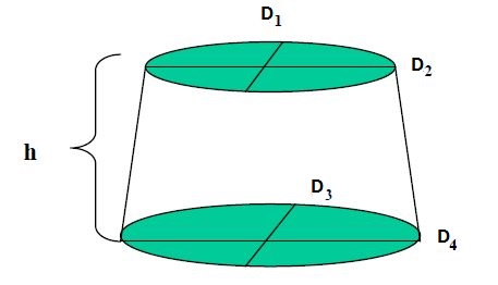
We’ll use the trees data set provided in {modeldata} (loaded with {tidymodels}) for demonstration purposes. Tree girth (in inches), height (in feet), and volume (in cubic feet) are provided. (Girth is somewhat like a measure of diameter.)
library(tidyverse)
library(tidymodels)
theme_set(theme_minimal(base_size = 14))data(trees)
trees <- as_tibble(trees)
trees## # A tibble: 31 × 3
## Girth Height Volume
## <dbl> <dbl> <dbl>
## 1 8.3 70 10.3
## 2 8.6 65 10.3
## 3 8.8 63 10.2
## 4 10.5 72 16.4
## 5 10.7 81 18.8
## 6 10.8 83 19.7
## 7 11 66 15.6
## 8 11 75 18.2
## 9 11.1 80 22.6
## 10 11.2 75 19.9
## # ℹ 21 more rowsNote that there is an analytical way to calculate tree volume from measures of diameter and height.

We observe that Girth is strongly correlated with Volume
trees %>%
  corrr::correlate()
## # A tibble: 3 × 4
## term Girth Height Volume
## <chr> <dbl> <dbl> <dbl>
## 1 Girth NA 0.519 0.967
## 2 Height 0.519 NA 0.598
## 3 Volume 0.967 0.598 NAShame on you 😉 if you didn’t guess I would make a scatter plot given a data set with two variables.
trees %>%
  ggplot(aes(x = Girth, y = Height)) +
  geom_point(aes(size = Volume))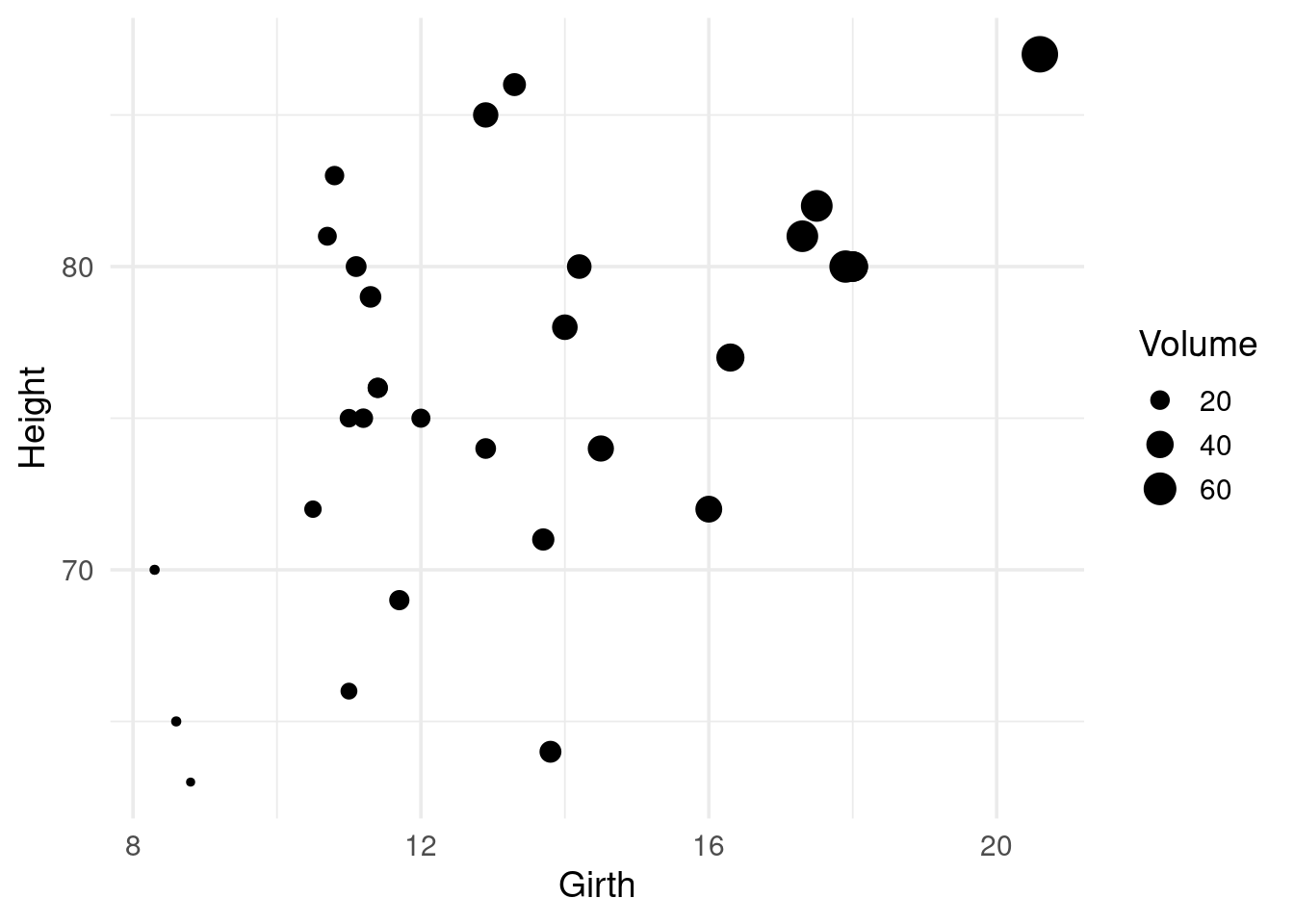
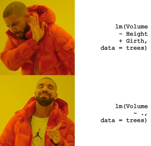
We can fit a linear regression model to predict Volume as a function of the other two features, using the formula syntax to save us from some typing.
reg_fit <- lm(Volume ~ ., data = trees)
reg_fit
##
## Call:
## lm(formula = Volume ~ ., data = trees)
##
## Coefficients:
## (Intercept) Girth Height
## -57.9877 4.7082 0.3393How would you write this without the formula syntax?
If we want to get fancy with our pipes (%>%), then we should wrap our formula with formula().
This due to the way . is interpreted by (%>%). The (%>%) passes the object on the left-hand side (lhs) to the first argument of a function call on the right-hand side (rhs).
Often you will want lhs to the rhs call at another position than the first. For this purpose you can use the dot (.) as placeholder. For example, y %>% f(x, .) is equivalent to f(x, y) and z %>% f(x, y, arg = .) is equivalent to f(x, y, arg = z). - magrittr/pipe
This would be confusing since within lm(), the . is interpreted as “all variables aside from the outcome”. This is why we explicitly call formula(). This allows us to pass the data object (trees) with the pipe to the data argument, below, not to the actual formula.
trees %>% lm(formula(Volume ~ .), data = .)##
## Call:
## lm(formula = formula(Volume ~ .), data = .)
##
## Coefficients:
## (Intercept) Girth Height
## -57.9877 4.7082 0.3393Interaction terms are easy to generate.
inter_fit <- lm(Volume ~ Girth * Height, data = trees)
inter_fit
##
## Call:
## lm(formula = Volume ~ Girth * Height, data = trees)
##
## Coefficients:
## (Intercept) Girth Height Girth:Height
## 69.3963 -5.8558 -1.2971 0.1347Same goes for polynomial terms. The use of the identity function, I(), allows us to apply literal math to the predictors.
poly_fit <- lm(Volume ~ Girth + I(Girth^2) + Height, data = trees)
poly_fit
##
## Call:
## lm(formula = Volume ~ Girth + I(Girth^2) + Height, data = trees)
##
## Coefficients:
## (Intercept) Girth I(Girth^2) Height
## -9.9204 -2.8851 0.2686 0.3764poly_fit3 <- lm(Volume ~ (.)^2, data = trees)
poly_fit3##
## Call:
## lm(formula = Volume ~ (.)^2, data = trees)
##
## Coefficients:
## (Intercept) Girth Height Girth:Height
## 69.3963 -5.8558 -1.2971 0.1347# There are only two predictors in this model so this produces the same results as
# inter_fit but if there were 3 there would be three individual
# effects and the combination of those effects as interaction depending on if the third
# variable is continuous or categoricalExcluding columns is intuitive.
no_height_fit <- lm(Volume ~ . - Height, data = trees)
no_height_fit
##
## Call:
## lm(formula = Volume ~ . - Height, data = trees)
##
## Coefficients:
## (Intercept) Girth
## -36.943 5.066The intercept term can be removed conveniently. This is just for illustrative purposes only. Removing the intercept is rarely done. In this particular case, it may make sense as it is impossible for a tree to have negative volume
no_intercept_fit <- lm(Volume ~ . + 0, data = trees)
no_intercept_fit
##
## Call:
## lm(formula = Volume ~ . + 0, data = trees)
##
## Coefficients:
## Girth Height
## 5.0440 -0.4773To illustrate another convenience provided by formulas, let’s add a categorical column.
trees2 <- trees
set.seed(42)
trees2$group = sample(toupper(letters[1:4]), size = nrow(trees2), replace = TRUE)
trees2
## # A tibble: 31 × 4
## Girth Height Volume group
## <dbl> <dbl> <dbl> <chr>
## 1 8.3 70 10.3 A
## 2 8.6 65 10.3 A
## 3 8.8 63 10.2 A
## 4 10.5 72 16.4 A
## 5 10.7 81 18.8 B
## 6 10.8 83 19.7 D
## 7 11 66 15.6 B
## 8 11 75 18.2 B
## 9 11.1 80 22.6 A
## 10 11.2 75 19.9 D
## # ℹ 21 more rowsEncoding the categories as separate features is done auto-magically with the formula syntax.
dummy_fit <- lm(Volume ~ ., data = trees2)
dummy_fit
##
## Call:
## lm(formula = Volume ~ ., data = trees2)
##
## Coefficients:
## (Intercept) Girth Height groupB groupC groupD
## -55.2921 4.6932 0.3093 -1.8367 -0.0497 0.6462Under the hood, this is done by model.matrix().
model.matrix(Volume ~ ., data = trees2) %>% head(10)## (Intercept) Girth Height groupB groupC groupD
## 1 1 8.3 70 0 0 0
## 2 1 8.6 65 0 0 0
## 3 1 8.8 63 0 0 0
## 4 1 10.5 72 0 0 0
## 5 1 10.7 81 1 0 0
## 6 1 10.8 83 0 0 1
## 7 1 11.0 66 1 0 0
## 8 1 11.0 75 1 0 0
## 9 1 11.1 80 0 0 0
## 10 1 11.2 75 0 0 1To visualize the inclusion of a polynomial:
dummy_fit3 <- lm(Volume ~ (.)^3, data = trees2)
dummy_fit3
##
## Call:
## lm(formula = Volume ~ (.)^3, data = trees2)
##
## Coefficients:
## (Intercept) Girth Height
## 60.087182 -5.435685 -1.137632
## groupB groupC groupD
## -17.115928 281.578642 -57.794217
## Girth:Height Girth:groupB Girth:groupC
## 0.126224 0.838817 -20.583875
## Girth:groupD Height:groupB Height:groupC
## 7.434342 0.152739 -3.639388
## Height:groupD Girth:Height:groupB Girth:Height:groupC
## 0.536103 -0.005086 0.266657
## Girth:Height:groupD
## -0.078695