20.6 Case Study - Patient Risk Profiles
This dataset contains 100 simulated patient’s medical history features and the predicted 1-year risk of 14 outcomes based on each patient’s medical history features. The predictions used real logistic regression models developed on a large real world healthcare dataset.
This data has been made available as #TidyTuesday dataset for week 43 - 2023 (https://github.com/rfordatascience/tidytuesday/blob/master/data/2023/2023-10-24/readme.md)
20.6.1 Loading necessary libraries
library(tidyverse)
library(tidymodels)
tidymodels::tidymodels_prefer()
20.6.2 Loading data
tuesdata <- tidytuesdayR::tt_load('2023-10-24')##
## Downloading file 1 of 1: `patient_risk_profiles.csv`raw <- tuesdata$patient_risk_profiles
# raw%>%glimpseraw[1:2,]20.6.3 Have a look at the data
Rearranging the data to have all the age group information as a column, then we count it to see all groups.
raw %>%
  column_to_rownames("personId") %>%
  pivot_longer(cols=contains("age group:"),
               names_to = "age_group_id",values_to = "age_group")%>%
  filter(!age_group==0)%>%
  count(age_group_id)
## # A tibble: 19 × 2
## age_group_id n
## <chr> <int>
## 1 age group: 0 - 4 5
## 2 age group: 5 - 9 4
## 3 age group: 10 - 14 4
## 4 age group: 15 - 19 5
## 5 age group: 20 - 24 11
## 6 age group: 25 - 29 4
## 7 age group: 30 - 34 3
## 8 age group: 35 - 39 5
## 9 age group: 40 - 44 2
## 10 age group: 45 - 49 9
## 11 age group: 50 - 54 4
## 12 age group: 55 - 59 7
## 13 age group: 60 - 64 10
## 14 age group: 65 - 69 3
## 15 age group: 70 - 74 2
## 16 age group: 75 - 79 11
## 17 age group: 80 - 84 4
## 18 age group: 85 - 89 4
## 19 age group: 90 - 94 3The same thing is done for the predicted risk.
raw %>%
  pivot_longer(cols = contains("predicted risk"),
               names_to = "predicted_risk_id",
               values_to = "predicted_risk")%>%
  count(predicted_risk_id)
## # A tibble: 14 × 2
## predicted_risk_id n
## <chr> <int>
## 1 predicted risk of Treatment resistant depression (TRD) 100
## 2 predicted risk of Acute pancreatitis, with No chronic or hereditary or… 100
## 3 predicted risk of Ankylosing Spondylitis 100
## 4 predicted risk of Autoimmune hepatitis 100
## 5 predicted risk of Dementia 100
## 6 predicted risk of Migraine 100
## 7 predicted risk of Multiple Sclerosis 100
## 8 predicted risk of Muscle weakness or injury 100
## 9 predicted risk of Parkinson's disease, inpatient or with 2nd diagnosis 100
## 10 predicted risk of Pulmonary Embolism 100
## 11 predicted risk of Restless Leg Syndrome 100
## 12 predicted risk of Sudden Hearing Loss, No congenital anomaly or middle… 100
## 13 predicted risk of Sudden Vision Loss, with no eye pathology causes 100
## 14 predicted risk of Ulcerative colitis 10020.6.4 Data wrangling
We transform the data into a more human-readable format, following the best practices for datasets.
Ensuring that each variable has its own column, each observation has its own row, and each type of observational unit forms a table.
dat <- raw %>%
    pivot_longer(cols = contains("predicted risk"),
               names_to = "predicted_risk_id",
               values_to = "predicted_risk")%>%
    pivot_longer(cols=contains("age group:"),
               names_to = "age_group_id",
               values_to = "age_group")%>%
    filter(!age_group==0)%>%
    select(-age_group)%>%
    pivot_longer(cols = contains("Sex"),
               names_to = "Sex_id",
               values_to = "Sex") %>%#count(Sex_id,Sex)
  filter(!Sex==0)%>%
  select(-Sex)%>%# dim
  pivot_longer(cols = contains("in prior year"),
               names_to = "Cause_id",
               values_to = "Cause")%>%
  filter(!Cause==0)%>%
  select(-Cause)%>%
   mutate(age_group_id=gsub("age group: ","",age_group_id),
         Sex_id=gsub("Sex = ","",Sex_id),
         Cause_id=gsub(" exposures in prior year","",Cause_id),
         predicted_risk_id=gsub("predicted risk of ","",predicted_risk_id),
         )%>%
  mutate(personId=as.factor(personId))


dat %>% head
## # A tibble: 6 × 6
## personId predicted_risk_id predicted_risk age_group_id Sex_id Cause_id
## <fct> <chr> <dbl> <chr> <chr> <chr>
## 1 1 Pulmonary Embolism 0.00000700 " 5 - 9" FEMALE Acetaminophen
## 2 1 Pulmonary Embolism 0.00000700 " 5 - 9" FEMALE Angina events …
## 3 1 Pulmonary Embolism 0.00000700 " 5 - 9" FEMALE ANTIEPILEPTICS…
## 4 1 Pulmonary Embolism 0.00000700 " 5 - 9" FEMALE Osteoarthritis…
## 5 1 Pulmonary Embolism 0.00000700 " 5 - 9" FEMALE Type 1 diabete…
## 6 1 Pulmonary Embolism 0.00000700 " 5 - 9" FEMALE Edema in prior…dat %>%
#count(predicted_risk_id)
filter(str_detect(predicted_risk_id,"Dementia"))%>% head## # A tibble: 6 × 6
## personId predicted_risk_id predicted_risk age_group_id Sex_id Cause_id
## <fct> <chr> <dbl> <chr> <chr> <chr>
## 1 1 Dementia 0.0000731 " 5 - 9" FEMALE Acetaminophen
## 2 1 Dementia 0.0000731 " 5 - 9" FEMALE Angina events i…
## 3 1 Dementia 0.0000731 " 5 - 9" FEMALE ANTIEPILEPTICS …
## 4 1 Dementia 0.0000731 " 5 - 9" FEMALE Osteoarthritis …
## 5 1 Dementia 0.0000731 " 5 - 9" FEMALE Type 1 diabetes…
## 6 1 Dementia 0.0000731 " 5 - 9" FEMALE Edema in prior …20.6.5 Data to use in the Model
Let’s use the raw data which provides dummy variables.
dementia <- raw %>%
  select(contains("Dementia"))%>%
  cbind(raw%>%select(!contains("Dementia")))%>%
  janitor::clean_names()
20.6.6 Spending Data
set.seed(24102023)
split <- initial_split(dementia,prop = 0.8)
train <- training(split)
test <- testing(split)
folds <- vfold_cv(train)
20.6.7 Preprocessing and Recipes
normalized_rec <- recipe(predicted_risk_of_dementia ~ ., train) %>%
  update_role("person_id",new_role = "id") %>%
  step_normalize(all_predictors()) %>%
  step_corr(all_predictors())%>%
step_zv(all_predictors())normalized_rec%>%
prep()%>%
juice()%>%
head## # A tibble: 6 × 100
## person_id age_group_10_14 age_group_15_19 age_group_20_24 age_group_65_69
## <dbl> <dbl> <dbl> <dbl> <dbl>
## 1 44 -0.159 -0.228 -0.376 -0.196
## 2 76 -0.159 -0.228 -0.376 -0.196
## 3 20 -0.159 -0.228 -0.376 -0.196
## 4 70 -0.159 -0.228 2.63 -0.196
## 5 14 -0.159 4.33 -0.376 -0.196
## 6 8 -0.159 4.33 -0.376 -0.196
## # ℹ 95 more variables: age_group_40_44 <dbl>, age_group_45_49 <dbl>,
## # age_group_55_59 <dbl>, age_group_85_89 <dbl>, age_group_75_79 <dbl>,
## # age_group_5_9 <dbl>, age_group_25_29 <dbl>, age_group_0_4 <dbl>,
## # age_group_70_74 <dbl>, age_group_50_54 <dbl>, age_group_60_64 <dbl>,
## # age_group_35_39 <dbl>, age_group_30_34 <dbl>, age_group_80_84 <dbl>,
## # age_group_90_94 <dbl>, sex_female <dbl>, sex_male <dbl>,
## # acetaminophen_exposures_in_prior_year <dbl>, …20.6.8 Make many models
Warning: All model specifications are the models used in Chapter 15. These models are not necessarily the first choice for this dataset but are used for educational purposes to build a diverse selection of different model types in order to select the best one.
We use 10 models:
1- Linear Regression: linear_reg_spec
2- Neural Network: nnet_spec
3- Mars (Motivation, Ability, Role Perception and Situational Factor): mars_spec
4A- Support Vector Machine: svm_r_spec
4B- Support Vector Machine poly: svm_p_spec
5- K-Nearest Neighbor: knn_spec
6- CART (Classification And Regression Tree): cart_spec
7- Bagging CART: bag_cart_spec
8- Random Forest: rf_spec
9- XGBoost: xgb_spec
10- Cubist: cubist_spec
library(rules)
library(baguette)

linear_reg_spec <-
   linear_reg(penalty = tune(),
              mixture = tune()) %>%
   set_engine("glmnet")

nnet_spec <-
   mlp(hidden_units = tune(),
       penalty = tune(),
       epochs = tune()) %>%
   set_engine("nnet", MaxNWts = 2600) %>%
   set_mode("regression")

mars_spec <-
   mars(prod_degree = tune()) %>%  #<- use GCV to choose terms
   set_engine("earth") %>%
   set_mode("regression")

svm_r_spec <-
   svm_rbf(cost = tune(),
           rbf_sigma = tune()) %>%
   set_engine("kernlab") %>%
   set_mode("regression")

svm_p_spec <-
   svm_poly(cost = tune(),
            degree = tune()) %>%
   set_engine("kernlab") %>%
   set_mode("regression")

knn_spec <-
   nearest_neighbor(neighbors = tune(),
                    dist_power = tune(),
                    weight_func = tune()) %>%
   set_engine("kknn") %>%
   set_mode("regression")

cart_spec <-
   decision_tree(cost_complexity = tune(),
                 min_n = tune()) %>%
   set_engine("rpart") %>%
   set_mode("regression")

bag_cart_spec <-
   bag_tree() %>%
   set_engine("rpart", times = 50L) %>%
   set_mode("regression")

rf_spec <-
   rand_forest(mtry = tune(),
               min_n = tune(),
               trees = 1000) %>%
   set_engine("ranger") %>%
   set_mode("regression")

xgb_spec <-
   boost_tree(tree_depth = tune(),
              learn_rate = tune(),
              loss_reduction = tune(),
              min_n = tune(),
              sample_size = tune(),
              trees = tune()) %>%
   set_engine("xgboost") %>%
   set_mode("regression")

cubist_spec <-
   cubist_rules(committees = tune(),
                neighbors = tune()) %>%
   set_engine("Cubist")
Here we update the nnet paramameters to a specified range.
nnet_param <-
   nnet_spec %>%
   extract_parameter_set_dials() %>%
   update(hidden_units = hidden_units(c(1, 27)))
20.6.9 Build the Workflow
First workflow_set with the normalized_rec. This will be applied to part of the models.
normalized <-
   workflow_set(
      preproc = list(normalized = normalized_rec),
      models = list(SVM_radial = svm_r_spec,
                    SVM_poly = svm_p_spec,
                    KNN = knn_spec,
                    neural_network = nnet_spec)
      )
normalized
## # A workflow set/tibble: 4 × 4
## wflow_id info option result
## <chr> <list> <list> <list>
## 1 normalized_SVM_radial <tibble [1 × 4]> <opts[0]> <list [0]>
## 2 normalized_SVM_poly <tibble [1 × 4]> <opts[0]> <list [0]>
## 3 normalized_KNN <tibble [1 × 4]> <opts[0]> <list [0]>
## 4 normalized_neural_network <tibble [1 × 4]> <opts[0]> <list [0]>Update the workflow_set with the nnet_param.
normalized <-
   normalized %>%
   option_add(param_info = nnet_param,
              id = "normalized_neural_network")
normalized
## # A workflow set/tibble: 4 × 4
## wflow_id info option result
## <chr> <list> <list> <list>
## 1 normalized_SVM_radial <tibble [1 × 4]> <opts[0]> <list [0]>
## 2 normalized_SVM_poly <tibble [1 × 4]> <opts[0]> <list [0]>
## 3 normalized_KNN <tibble [1 × 4]> <opts[0]> <list [0]>
## 4 normalized_neural_network <tibble [1 × 4]> <opts[1]> <list [0]>20.6.9.1 Add a no pre-processing recipe
Add a simple recipe using workflow_variables() function to search for the response variable relationship across all predictors without preprocessing steps.
Set the second workflow_set with the no_pre_proc recipe. This will be applied to the remaining part of the models.
model_vars <-
   workflow_variables(outcomes = predicted_risk_of_dementia,
                      predictors = everything())

no_pre_proc <-
   workflow_set(
      preproc = list(simple = model_vars),
      models = list(MARS = mars_spec,
                    CART = cart_spec,
                    CART_bagged = bag_cart_spec,
                    RF = rf_spec,
                    boosting = xgb_spec,
                    Cubist = cubist_spec)
      )
no_pre_proc
## # A workflow set/tibble: 6 × 4
## wflow_id info option result
## <chr> <list> <list> <list>
## 1 simple_MARS <tibble [1 × 4]> <opts[0]> <list [0]>
## 2 simple_CART <tibble [1 × 4]> <opts[0]> <list [0]>
## 3 simple_CART_bagged <tibble [1 × 4]> <opts[0]> <list [0]>
## 4 simple_RF <tibble [1 × 4]> <opts[0]> <list [0]>
## 5 simple_boosting <tibble [1 × 4]> <opts[0]> <list [0]>
## 6 simple_Cubist <tibble [1 × 4]> <opts[0]> <list [0]>20.6.9.2 All Workflows
all_workflows <-
   bind_rows(no_pre_proc, normalized) %>%
   # Make the workflow ID's a little more simple:
   mutate(wflow_id = gsub("(simple_)|(normalized_)", "", wflow_id))
all_workflows
## # A workflow set/tibble: 10 × 4
## wflow_id info option result
## <chr> <list> <list> <list>
## 1 MARS <tibble [1 × 4]> <opts[0]> <list [0]>
## 2 CART <tibble [1 × 4]> <opts[0]> <list [0]>
## 3 CART_bagged <tibble [1 × 4]> <opts[0]> <list [0]>
## 4 RF <tibble [1 × 4]> <opts[0]> <list [0]>
## 5 boosting <tibble [1 × 4]> <opts[0]> <list [0]>
## 6 Cubist <tibble [1 × 4]> <opts[0]> <list [0]>
## 7 SVM_radial <tibble [1 × 4]> <opts[0]> <list [0]>
## 8 SVM_poly <tibble [1 × 4]> <opts[0]> <list [0]>
## 9 KNN <tibble [1 × 4]> <opts[0]> <list [0]>
## 10 neural_network <tibble [1 × 4]> <opts[1]> <list [0]>20.6.10 Tuning: Grid and Race
Set up a parallel processing set to use all cores in your computer and faster the computation.
doParallel::registerDoParallel()grid_ctrl <-
control_grid(
save_pred = TRUE,
parallel_over = "everything",
save_workflow = TRUE
)
grid_results <-
all_workflows %>%
workflow_map(
seed = 24102023,
resamples = folds,
# warning this is for educational purposes
grid = 5, # grid should be higher
control = grid_ctrl
)
# saveRDS(grid_results,file="data/grid_results.rds")
# grid_results <- readRDS("data/grid_results.rds")grid_results %>%
rank_results() %>%
filter(.metric == "rmse") %>%
select(model, .config, rmse = mean, rank)autoplot(
grid_results,
rank_metric = "rmse", # <- how to order models
metric = "rmse", # <- which metric to visualize
select_best = TRUE # <- one point per workflow
) +
geom_text(aes(y = mean-0.02,
label = wflow_id),
angle = 90,
hjust = 1) +
lims(y = c(-0.05, 0.1)) +
theme(legend.position = "none")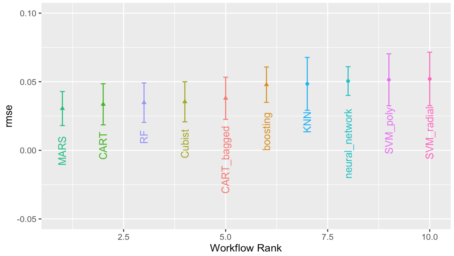
autoplot(grid_results, id = "Cubist", metric = "rmse")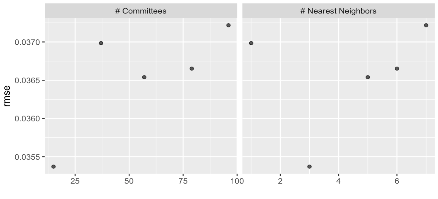
20.6.10.1 Racing
library(finetune)

race_ctrl <-
   control_race(
      save_pred = TRUE,
      parallel_over = "everything",
      save_workflow = TRUE
   )

race_results <-
   all_workflows %>%

  workflow_map(
      "tune_race_anova",
      seed = 1503,
      resamples = folds,
      # warning this is for educational purposes
      grid = 5, # grid should be higher
      control = race_ctrl
   )

# saveRDS(race_results,file="data/race_results.rds")
# race_results <- readRDS("data/race_results.rds")autoplot(
race_results,
rank_metric = "rmse",
metric = "rmse",
select_best = TRUE
) +
geom_text(aes(y = mean - 0.02,
label = wflow_id),
angle = 90,
hjust = 1) +
lims(y = c(-0.05, 0.1)) +
theme(legend.position = "none")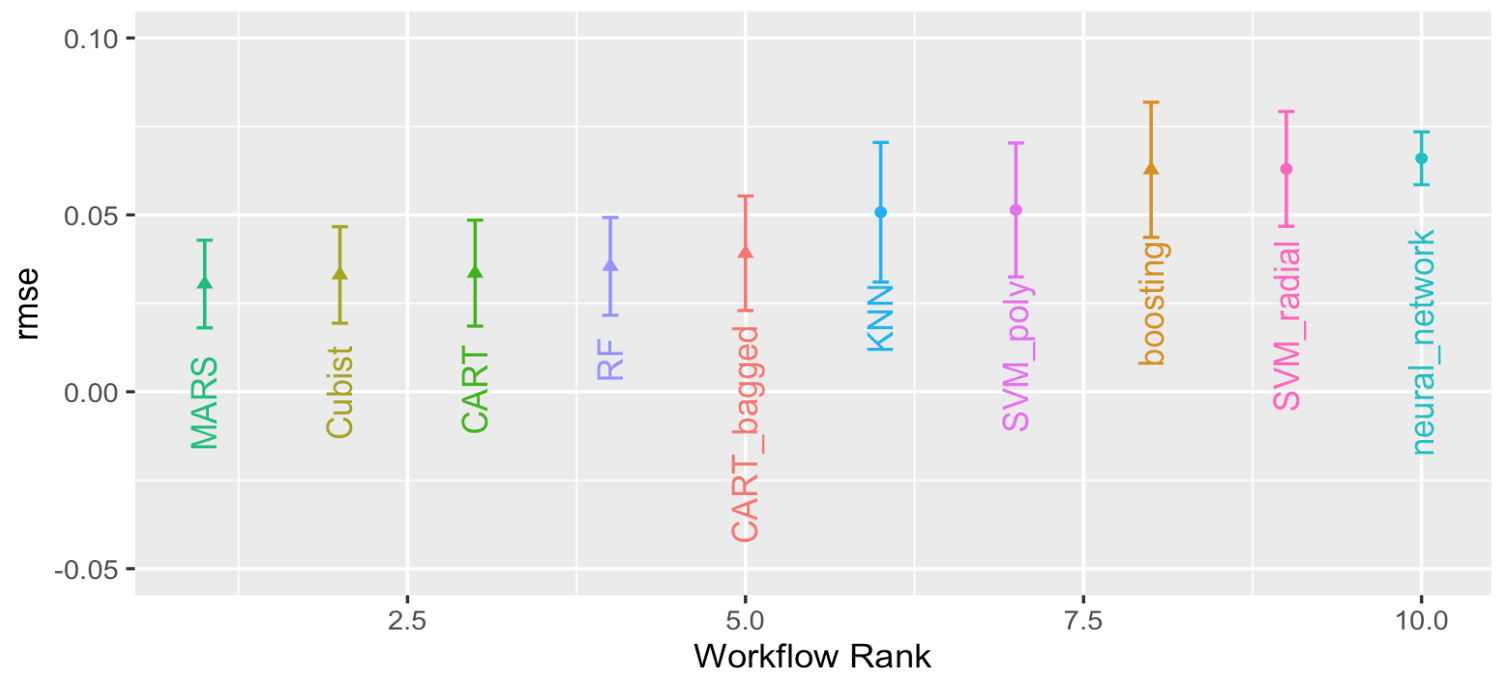
20.6.11 Stacking (Ensembles of models)
library(stacks)
#?stacks
dementia_stack <-
  stacks() %>%
add_candidates(race_results)set.seed(25102023)
ens <- blend_predictions(dementia_stack)
autoplot(ens)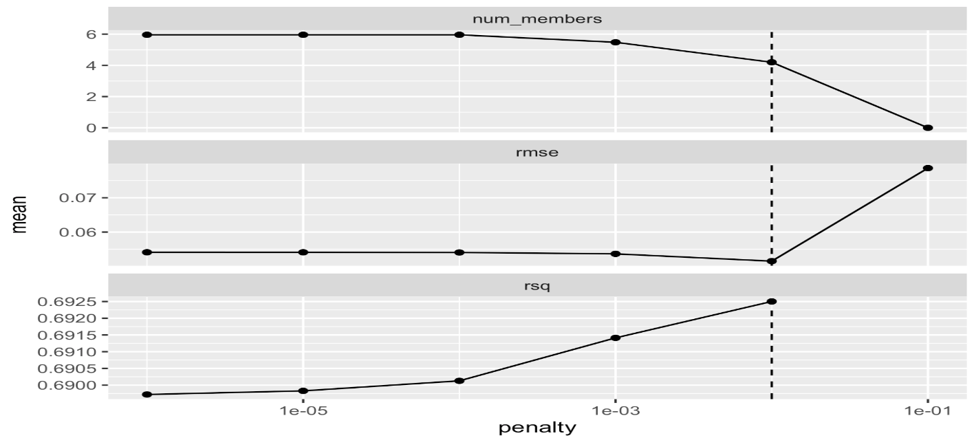
ens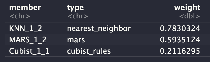
set.seed(25102023)
ens2 <- blend_predictions(dementia_stack,
                         penalty = 10^seq(-2, -0.5, length = 20))
autoplot(ens2)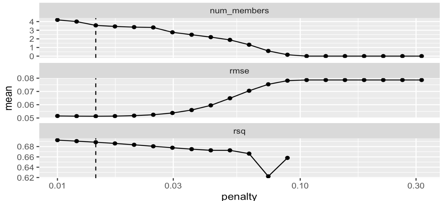
Let’s check which model provide the largest contributions to the ensemble.
autoplot(ens2, "weights") +
  geom_text(aes(x = weight + 0.01,
                label = model), hjust = 0) +
  theme(legend.position = "none") +
  lims(x = c(-0.01, 1))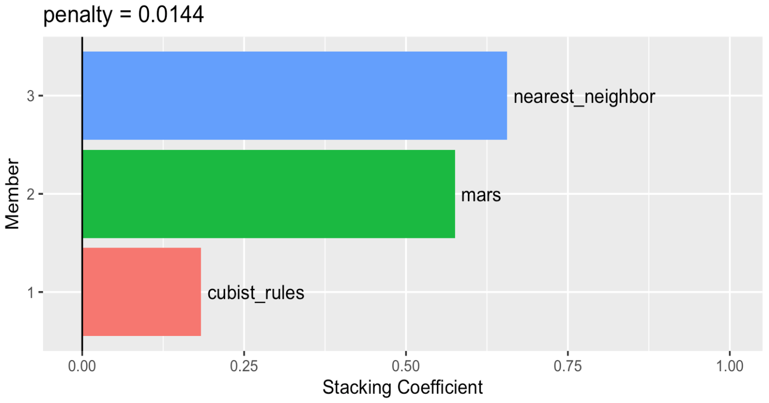
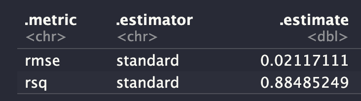
ens_fit <- fit_members(ens2)reg_metrics <- metric_set(rmse, rsq)
ens_test_pred <-
predict(ens_fit, test) %>%
bind_cols(test)
ens_test_pred %>%
reg_metrics(predicted_risk_of_dementia, .pred)