19.1 Equivocal Results

What the heck is this? Loosely, equivacol results are a range of results indicating that the prediction should not be reported.

Let’s take a soccer example. (Data courtesy of 538.)

df <- 
  here::here('data', 'spi_matches_latest.csv') %>% 
  read_csv() %>% 
  drop_na(score1) %>% 
  mutate(w1 = ifelse(score1 > score2, 'yes', 'no') %>% factor()) %>% 
  select(
    w1, season, matches('(team|spi|prob|importance)[12]'), probtie
  ) %>% 
  # we need this as  feature, so it can't be NA
  drop_na(importance1)

# much more data in 2021 season than in older seasons, so use older seasons as test set
trn <- df %>% filter(season == 2021) %>% select(-season)
tst <- df %>% filter(season != 2021) %>% select(-season)
trn %>% count(w1)

## # A tibble: 2 × 2
##   w1        n
##   <fct> <int>
## 1 no     1376
## 2 yes    1054

tst %>% count(w1)

## # A tibble: 2 × 2
##   w1        n
##   <fct> <int>
## 1 no      248
## 2 yes     227

fit <-
  logistic_reg() %>% 
  set_engine('glm') %>% 
  # 2 variables cuz dumb humans like 2-D plots
  fit(w1 ~ spi1 + importance1, data = trn)
fit %>% tidy()

## # A tibble: 3 × 5
##   term        estimate std.error statistic  p.value
##   <chr>          <dbl>     <dbl>     <dbl>    <dbl>
## 1 (Intercept) -0.742     0.107       -6.92 4.50e-12
## 2 spi1         0.0100    0.00259      3.86 1.13e- 4
## 3 importance1  0.00381   0.00250      1.52 1.27e- 1

predict_stuff <- function(fit, set) {
  bind_cols(
    fit %>% 
      predict(set),
    fit %>% 
      predict(set, type = 'prob'),
    fit %>% 
      predict(set, type = 'conf_int', std_error = TRUE),
    set
  )
}

preds_tst <- fit %>% predict_stuff(tst)

How’s the model accuracy?

preds_tst %>% 
  accuracy(estimate = .pred_class, truth = w1)

## # A tibble: 1 × 3
##   .metric  .estimator .estimate
##   <chr>    <chr>          <dbl>
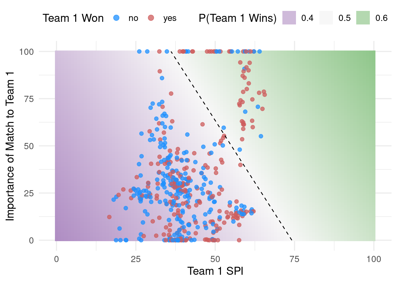
## 1 accuracy binary         0.579

Seems reasonable… so maybe modeling soccer match outcomes with 2 variables ain’t so bad, eh?

Observe the fitted class boundary. (Confidence intervals shown instead of prediction intervals because I didn’t want to use stan… Max please forgive me.)

Use the {probably} package!

lvls <- levels(preds_tst$w1)

preds_tst_eqz <- 
  preds_tst %>% 
  mutate(.pred_with_eqz = make_two_class_pred(.pred_yes, lvls, buffer = 0.025))

preds_tst_eqz %>% count(.pred_with_eqz)

## # A tibble: 3 × 2
##   .pred_with_eqz     n
##       <clss_prd> <int>
## 1           [EQ]    50
## 2             no    48
## 3            yes   377

Look at how make_two_class_pred changes our confusion matrix.

# All data
preds_tst_eqz %>% conf_mat(w1, .pred_class) %>% autoplot('heatmap')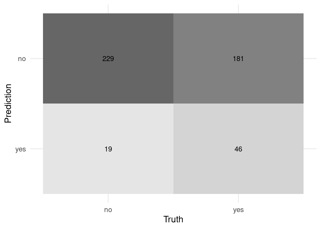

# Reportable results only
preds_tst_eqz %>% conf_mat(w1, .pred_with_eqz) %>% autoplot('heatmap')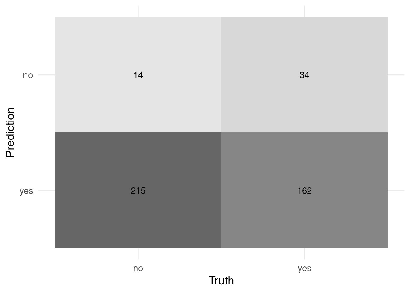

Does the equivocal zone help improve accuracy? How sensitive is accuracy and our reportable rate to the width of the buffer?

eq_zone_results <- function(buffer) {
  preds_tst_eqz <- 
    preds_tst %>% 
    mutate(.pred_with_eqz = make_two_class_pred(.pred_no, lvls, buffer = buffer))
  acc <- preds_tst_eqz %>% accuracy(w1, .pred_with_eqz)
  rep_rate <- reportable_rate(preds_tst_eqz$.pred_with_eqz)
  tibble(accuracy = acc$.estimate, reportable = rep_rate, buffer = buffer)
}

map_dfr(seq(0, 0.15, length.out = 40), eq_zone_results) %>% 
  pivot_longer(c(-buffer)) %>% 
  ggplot(aes(x = buffer, y = value, col = name)) + 
  geom_step(size = 1.2, alpha = 0.8) + 
  labs(y = NULL)

How does the standard error look across the feature space

Makes sense… we’re more uncertain for cases outside of the normal boundary of our data.