6.1 - Why regularize?

ames <- AmesHousing::make_ames()

# Stratified sampling with the rsample package
set.seed(123)  # for reproducibility
split  <- initial_split(ames, prop = 0.7, strata = "Sale_Price")
ames_train  <- training(split)
ames_test   <- testing(split)

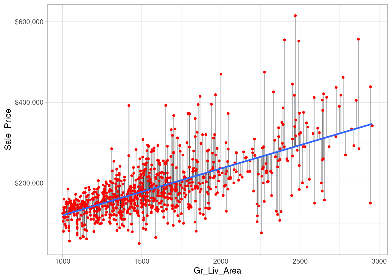
Create an OLS model with Sale_Price ~ Gr_Liv_Area

ames_sub <- ames_train %>%
     filter(Gr_Liv_Area > 1000 & Gr_Liv_Area < 3000) %>%
     sample_frac(0.5)

model1 <- lm(Sale_Price ~ Gr_Liv_Area, data = ames_sub)

model1 %>%
     broom::augment() %>%
     ggplot(aes(Gr_Liv_Area, Sale_Price)) + 
     geom_segment(aes(x = Gr_Liv_Area, y = Sale_Price,
                      xend = Gr_Liv_Area, yend = .fitted), 
                  alpha = 0.3) +
     geom_point(size = 1, color = "red") +
     geom_smooth(se = FALSE, method = "lm") +
     scale_y_continuous(labels = scales::dollar)

## `geom_smooth()` using formula = 'y ~ x'

The objective function being minimized can be written as:

\[\begin{equation} \operatorname{minimize}\left(S S E=\sum_{i=1}^n\left(y_i-\hat{y}_i\right)^2\right) \end{equation}\]

• For more complex datasets, OLS assumptions can be violated, such as the number of predictors (\(p\)) greater than the number of observations (\(n\)). Also, the presence of multicollinearity increases with the addition of predictors.

• A solution to the above scenario is the use of penalized models or shrinkage methods to constrain the total size of all the coefficient estimates.

• This constraint helps to reduce the magnitude and fluctuations of the coefficients and will reduce the variance of our model (at the expense of no longer being unbiased (a reasonable compromise).

• The objective function of a regularized regression model is similar to OLS, albeit with a penalty term \(P\).

\[\begin{equation} \operatorname{minimize}(S S E + P) \end{equation}\]

There are three common penalty parameters we can implement:

• Ridge;

• Lasso;

• ElasticNet, which is a combination of ridge and lasso