3.5 Numeric feature engineering

Numeric features can create a host of problems for certain models when their distributions are skewed, contain outliers, or have a wide range in magnitudes.

Tree-based models are quite immune to these types of problems in the feature space, but many other models (e.g., GLMs, regularized regression, KNN, support vector machines, neural networks) can be greatly hampered by these issues.

Normalizing and standardizing heavily skewed features can help minimize these concerns.

• Skewness

Similar to the process discussed to normalize target variables, parametric models that have distributional assumptions (e.g., GLMs, and regularized models) can benefit from minimizing the skewness of numeric features.

• Standardization

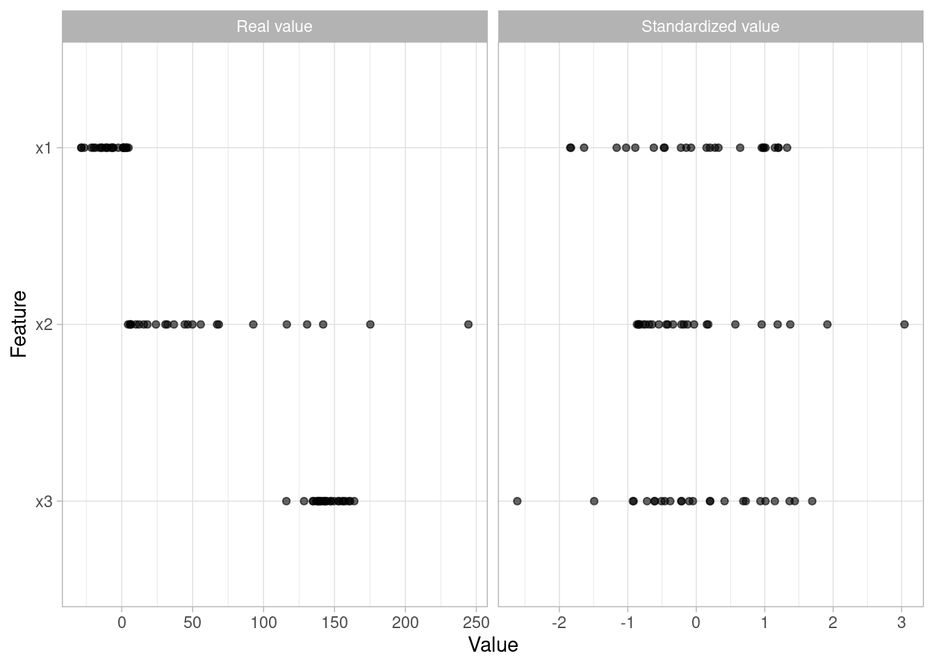
We must also consider the scale on which the individual features are measured. What are the largest and smallest values across all features and do they span several orders of magnitude? Models that incorporate smooth functions of input features are sensitive to the scale of the inputs.

set.seed(123)
x1 <- tibble(
  variable = "x1",
  `Real value` = runif(25, min = -30, max = 5),
  `Standardized value` = scale(`Real value`) %>% as.numeric()
)

set.seed(456)
x2 <- tibble(
  variable = "x2",
  `Real value` = rlnorm(25, log(25)),
  `Standardized value` = scale(`Real value`) %>% as.numeric()
)

set.seed(789)
x3 <- tibble(
  variable = "x3",
  `Real value` = rnorm(25, 150, 15),
  `Standardized value` = scale(`Real value`) %>% as.numeric()
)

x1 %>%
  bind_rows(x2) %>%
  bind_rows(x3) %>%
  gather(key, value, -variable) %>%
  mutate(variable = factor(variable, levels = c("x3", "x2", "x1"))) %>%
  ggplot(aes(value, variable)) +
    geom_point(alpha = .6) +
    facet_wrap(~ key, scales = "free_x") +
    ylab("Feature") +
    xlab("Value")