6.3 - Implementation

We’ll us the glmnet package for the regularized regression models.

# Create training  feature matrices
# we use model.matrix(...)[, -1] to discard the intercept
X <- model.matrix(Sale_Price ~ ., ames_train)[, -1]

# transform y with log transformation
Y <- log(ames_train$Sale_Price)

To apply a regularized model we can use the glmnet::glmnet() function. The alpha parameter tells glmnet to perform a ridge (alpha = 0), lasso (alpha = 1), or elastic net (0 < alpha < 1) model.

ridge <- glmnet(
  x = X,
  y = Y,
  alpha = 0
)

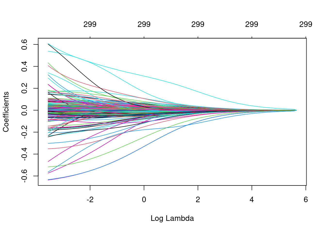
plot(ridge, xvar = "lambda")

# lambdas applied to penalty parameter
ridge$lambda %>% head()

## [1] 285.7769 260.3893 237.2570 216.1798 196.9749 179.4762

ridge$lambda %>% tail()

## [1] 0.04550377 0.04146134 0.03777803 0.03442193 0.03136398 0.02857769

# small lambda results in large coefficients
coef(ridge)[c("Latitude", "Overall_QualVery_Excellent"), 100]

##                   Latitude Overall_QualVery_Excellent 
##                 0.60703722                 0.09344684

# large lambda results in small coefficients
coef(ridge)[c("Latitude", "Overall_QualVery_Excellent"), 1]

##                   Latitude Overall_QualVery_Excellent 
##               6.115930e-36               9.233251e-37

At this point, we do not understand how much improvement we are experiencing in our loss function across various λ values.