16.9 LIME
Local Interpretable Model-agnostic Explanations (LIME) is an algorithm that helps explain individual predictions which assumes that every complex model is linear on a local scale after applying the next steps:
- Permute your training data to create new data points that are similar to the original one, but with some changes in the feature values.
- Compute proximity measure (e.g., 1 - distance) between the observation of interest and each of the permuted observations.
- Apply selected machine learning model to predict outcomes of permuted data.
- Select \(m\) number of features to best describe predicted outcomes.
- Fit a simple model (LASSO) to the permuted data, explaining the complex model outcome with \(m\) features from the permuted data weighted by its similarity to the original observation.
- Use the resulting feature weights to explain local behavior.
Source: https://ema.drwhy.ai/LIME.html
16.9.1 Implementation
In R the algorithm has been written in iml, lime and DALEX. Let’s use the iml one:
- Create a list that contains the fitted machine learning model and the feature distributions for the training data.
# Create explainer object
components_lime <- lime::lime(
  x = features,
  model = ensemble_tree,
  n_bins = 10
)

class(components_lime)
## [1] "data_frame_explainer" "explainer"            "list"

summary(components_lime)
##                      Length Class              Mode
## model                 1     H2ORegressionModel S4
## preprocess            1     -none-             function
## bin_continuous        1     -none-             logical
## n_bins                1     -none-             numeric
## quantile_bins         1     -none-             logical
## use_density           1     -none-             logical
## feature_type         80     -none-             character
## bin_cuts             80     -none-             list
## feature_distribution 80 -none- list- Perform the LIME algorithm using the
lime::explain()function on the observation(s) of interest.
# Use LIME to explain previously defined instances: high_ob and low_ob
lime_explanation <- lime::explain(
# Observation(s) you want to create local explanations for
x = rbind(high_ob, low_ob),
# Takes the explainer object created by lime::lime()
explainer = components_lime,
# The number of permutations to create for each observation in x
n_permutations = 5000,
# The distance function to use `?dist()`
dist_fun = "gower",
# the distance measure to a similarity score
kernel_width = 0.25,
# The number of features to best describe
# the predicted outcomes
n_features = 10,
feature_select = "highest_weights"
)
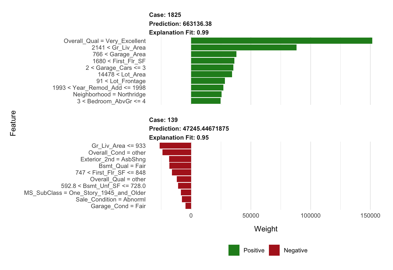
glimpse(lime_explanation)
## Observations: 20
## Variables: 11
## $ model_type <chr> "regression", "regression", "regression", "regr…
## $ case <chr> "1825", "1825", "1825", "1825", "1825", "1825",…
## $ model_r2 <dbl> 0.41661172, 0.41661172, 0.41661172, 0.41661172,…
## $ model_intercept <dbl> 186253.6, 186253.6, 186253.6, 186253.6, 186253.…
## $ model_prediction <dbl> 406033.5, 406033.5, 406033.5, 406033.5, 406033.…
## $ feature <chr> "Gr_Liv_Area", "Overall_Qual", "Total_Bsmt_SF",…
## $ feature_value <int> 3627, 8, 1930, 35760, 1796, 1831, 3, 14, 1, 3, …
## $ feature_weight <dbl> 55254.859, 50069.347, 40261.324, 20430.128, 193…
## $ feature_desc <chr> "2141 < Gr_Liv_Area", "Overall_Qual = Very_Exce…
## $ data <list> [[Two_Story_1946_and_Newer, Residential_Low_De…
## $ prediction <dbl> 663136.38, 663136.38, 663136.38, 663136.38, 663…
plot_features(lime_explanation, ncol = 1)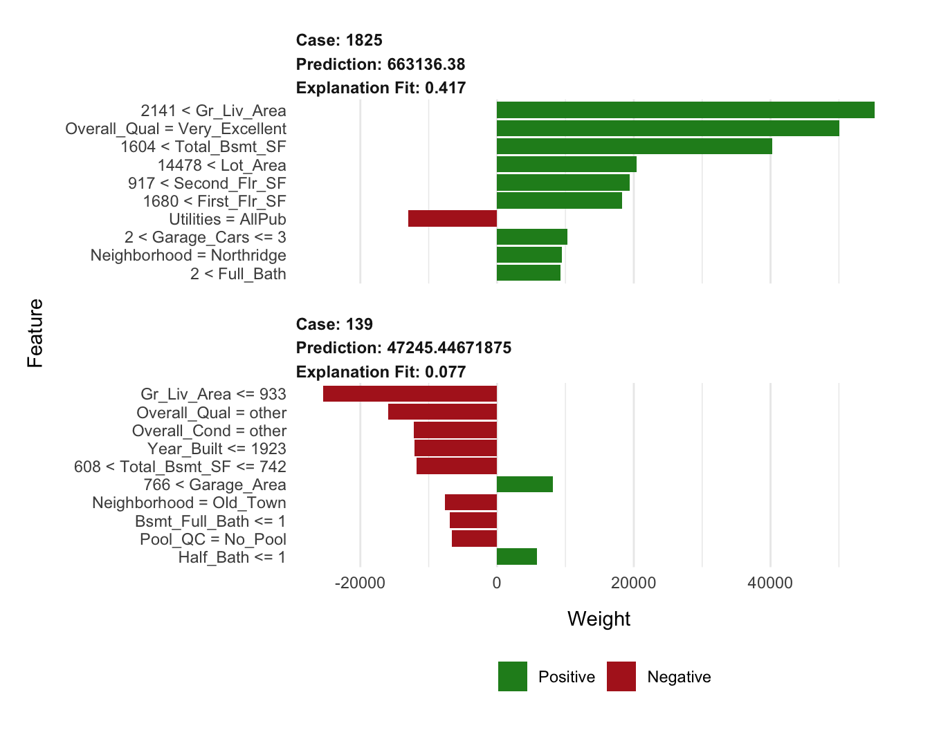
- Tune the LIME algorithm.
 # Tune the LIME algorithm a bit
lime_explanation2 <- explain(
  x = rbind(high_ob, low_ob),
  explainer = components_lime,
  n_permutations = 5000,
  dist_fun = "euclidean",
  kernel_width = 0.75,
  n_features = 10,
  feature_select = "lasso_path"
)

# Plot the results
plot_features(lime_explanation2, ncol = 1)