6.5 - Feature interpretation

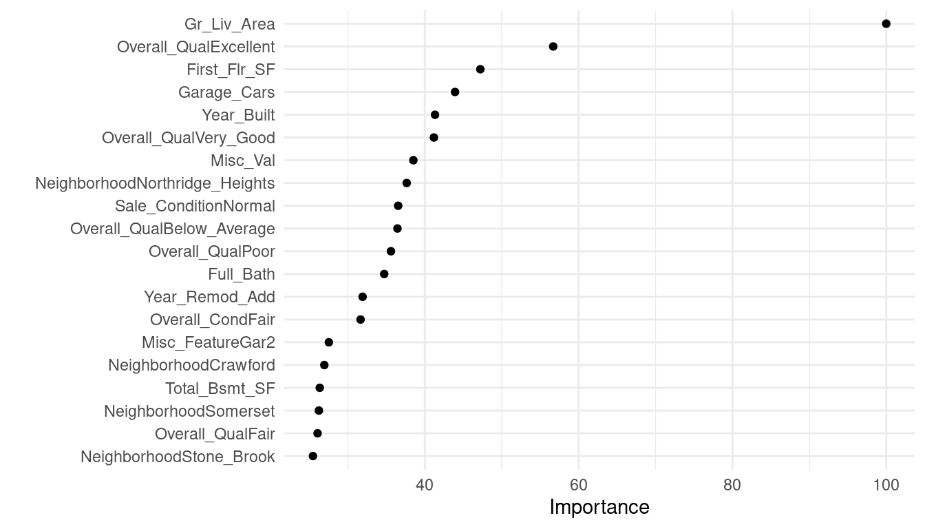
Variable importance for regularized models provides a similar interpretation as in linear (or logistic) regression. Importance is determined by magnitude of the standardized coefficients.

vip(cv_glmnet, num_features = 20, geom = 'point') + 
     theme_minimal()

Figure 6.3: Top 20 most important variables for the optimal regularized regression model.

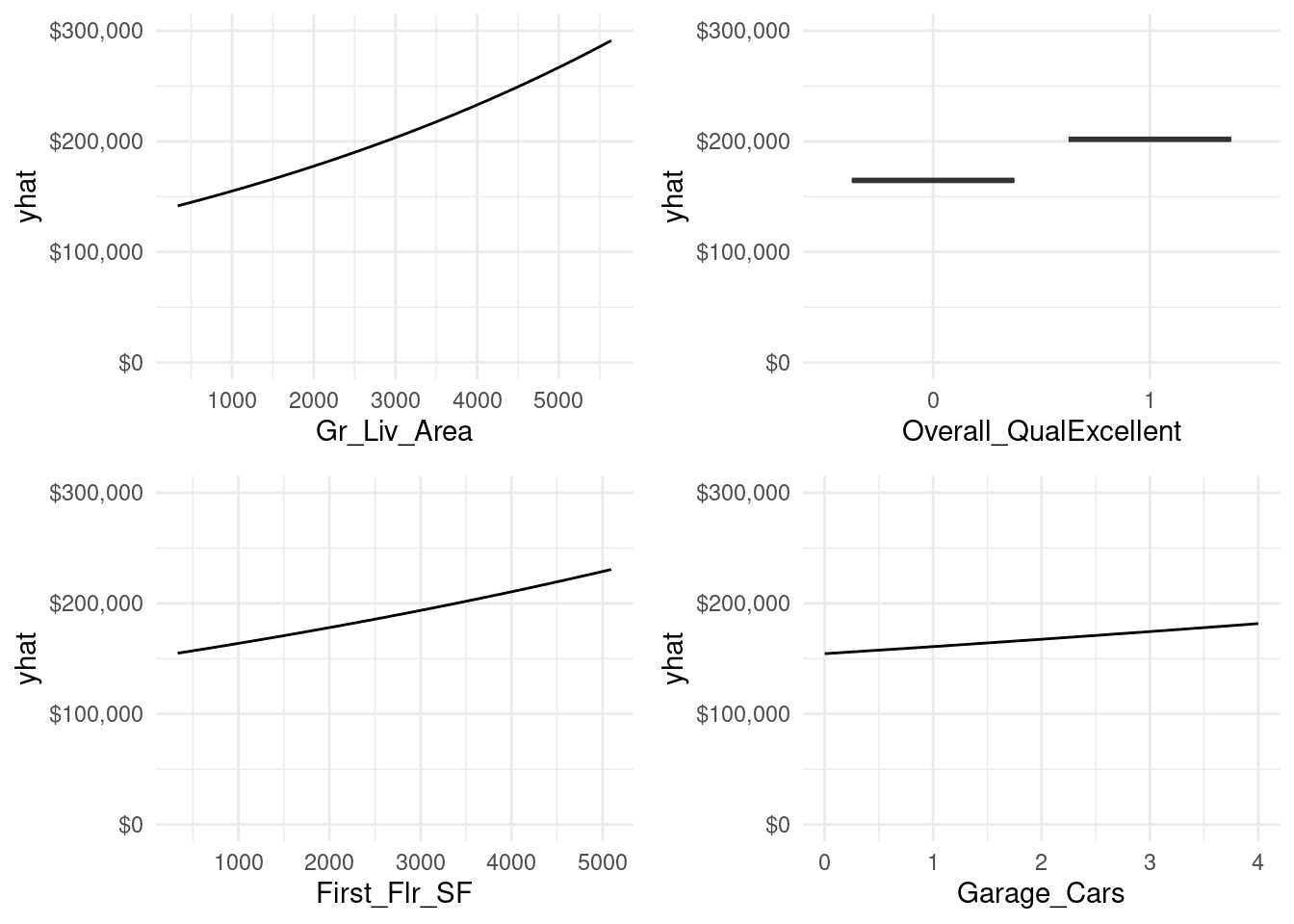
Similar to linear and logistic regression, the relationship between the features and response is monotonic linear. However, since we modeled our response with a log transformation, the estimated relationships will still be monotonic but non-linear on the original response scale.

theme_set(theme_minimal())

p1 <- pdp::partial(cv_glmnet, pred.var = "Gr_Liv_Area", grid.resolution = 20) %>%
  mutate(yhat = exp(yhat)) %>%
  ggplot(aes(Gr_Liv_Area, yhat)) +
  geom_line() +
  scale_y_continuous(limits = c(0, 300000), labels = scales::dollar)

p2 <- pdp::partial(cv_glmnet, pred.var = "Overall_QualExcellent") %>%
  mutate(
    yhat = exp(yhat),
    Overall_QualExcellent = factor(Overall_QualExcellent)
    ) %>%
  ggplot(aes(Overall_QualExcellent, yhat)) +
  geom_boxplot() +
  scale_y_continuous(limits = c(0, 300000), labels = scales::dollar)

p3 <- pdp::partial(cv_glmnet, pred.var = "First_Flr_SF", grid.resolution = 20) %>%
  mutate(yhat = exp(yhat)) %>%
  ggplot(aes(First_Flr_SF, yhat)) +
  geom_line() +
  scale_y_continuous(limits = c(0, 300000), labels = scales::dollar)

p4 <- pdp::partial(cv_glmnet, pred.var = "Garage_Cars") %>%
  mutate(yhat = exp(yhat)) %>%
  ggplot(aes(Garage_Cars, yhat)) +
  geom_line() +
  scale_y_continuous(limits = c(0, 300000), labels = scales::dollar)

gridExtra::grid.arrange(p1, p2, p3, p4, nrow = 2)

Figure 6.4: Partial dependence plots for the first four most important variables.

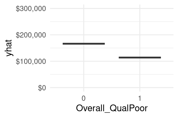
However, not that one of the top 20 most influential variables is Overall_QualPoor.

When a home has an overall quality rating of poor we see that the average predicted sales price decreases versus when it has some other overall quality rating.

Consequently, its important to not only look at the variable importance ranking, but also observe the positive or negative nature of the relationship.

pdp::partial(cv_glmnet, pred.var = "Overall_QualPoor") %>%
  mutate(
    yhat = exp(yhat),
    Overall_QualPoor = factor(Overall_QualPoor)
    ) %>%
  ggplot(aes(Overall_QualPoor, yhat)) +
  geom_boxplot() +
  scale_y_continuous(limits = c(0, 300000), labels = scales::dollar) + 
     theme_minimal()

Figure 6.5: Partial dependence plot for when overall quality of a home is (1) versus is not poor (0).