6.4 - Tuning

Recall that λ is a tuning parameter that helps to control our model from over-fitting to the training data.

We use k-fold CV to identify the optimal λ.

# Apply CV ridge regression to Ames data
ridge <- cv.glmnet(
  x = X,
  y = Y,
  alpha = 0
)

# Apply CV lasso regression to Ames data
lasso <- cv.glmnet(
  x = X,
  y = Y,
  alpha = 1
)

# plot results
par(mfrow = c(1, 2))
plot(ridge, main = "Ridge penalty\n\n")
plot(lasso, main = "Lasso penalty\n\n")

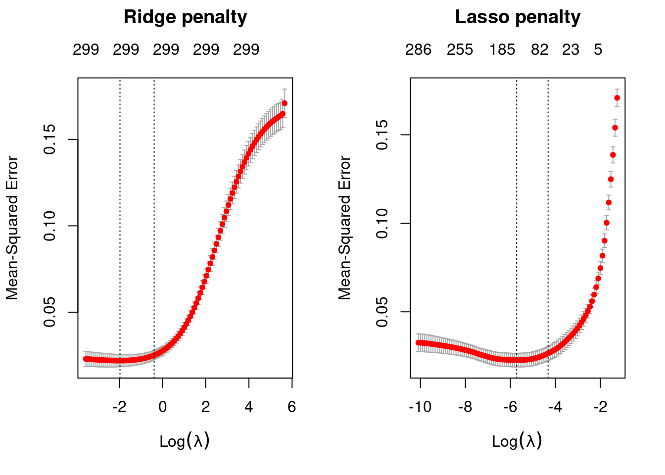
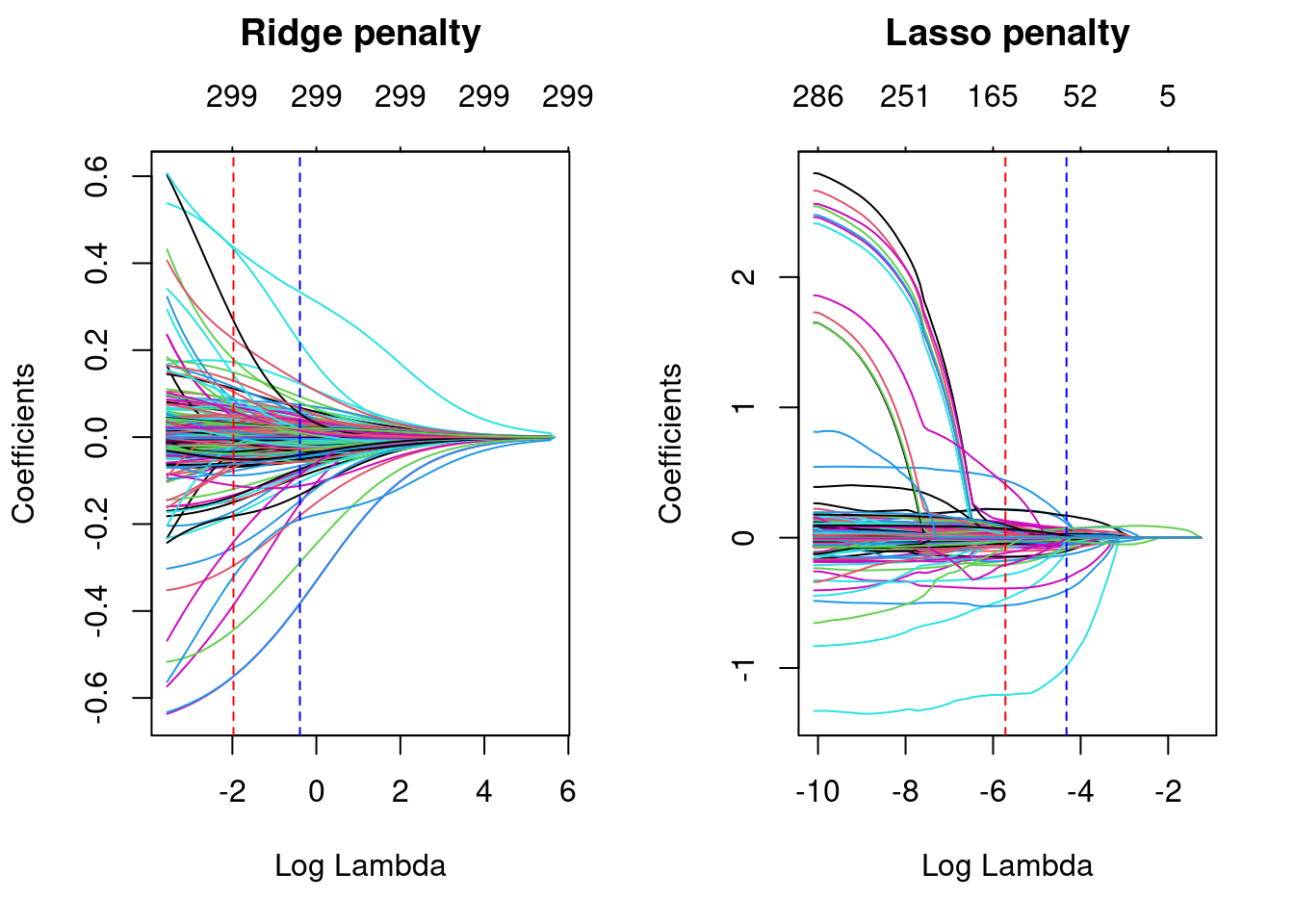
Ridge regression does not force any variables to exactly zero so all features will remain in the model but we see the number of variables retained in the lasso model decrease as the penalty increases.

The first and second vertical dashed lines represent the λ value with the minimum MSE and the largest λ value within one standard error of it. The minimum MSE for our ridge model is 0.02194817 (produced when λ= 0.1389619), whereas the minimum MSE for our lasso model is 0.0220374 (produced when λ= 0.00328574).

# Ridge model
min(ridge$cvm)       # minimum MSE

## [1] 0.02194817

ridge$lambda.min     # lambda for this min MSE

## [1] 0.1389619

ridge$cvm[ridge$lambda == ridge$lambda.1se]  # 1-SE rule

## [1] 0.02512028

ridge$lambda.1se  # lambda for this MSE

## [1] 0.6757165

# Lasso model
min(lasso$cvm)       # minimum MSE

## [1] 0.02270374

lasso$lambda.min     # lambda for this min MSE

## [1] 0.00328574

lasso$cvm[lasso$lambda == lasso$lambda.1se]  # 1-SE rule

## [1] 0.02653887

lasso$lambda.1se  # lambda for this MSE

## [1] 0.01326459

Above, we saw that both ridge and lasso penalties provide similar MSEs; however, these plots illustrate that ridge is still using all 299 features whereas the lasso model can get a similar MSE while reducing the feature set from 294 down to 135.

However, there will be some variability with this MSE and we can reasonably assume that we can achieve a similar MSE with a slightly more constrained model that uses only 69 features.

Although this lasso model does not offer significant improvement over the ridge model, we get approximately the same accuracy by using only 69 features!

# Ridge model
ridge_min <- glmnet(
  x = X,
  y = Y,
  alpha = 0
)

# Lasso model
lasso_min <- glmnet(
  x = X,
  y = Y,
  alpha = 1
)

par(mfrow = c(1, 2))
# plot ridge model
plot(ridge_min, xvar = "lambda", main = "Ridge penalty\n\n")
abline(v = log(ridge$lambda.min), col = "red", lty = "dashed")
abline(v = log(ridge$lambda.1se), col = "blue", lty = "dashed")

# plot lasso model
plot(lasso_min, xvar = "lambda", main = "Lasso penalty\n\n")
abline(v = log(lasso$lambda.min), col = "red", lty = "dashed")
abline(v = log(lasso$lambda.1se), col = "blue", lty = "dashed")

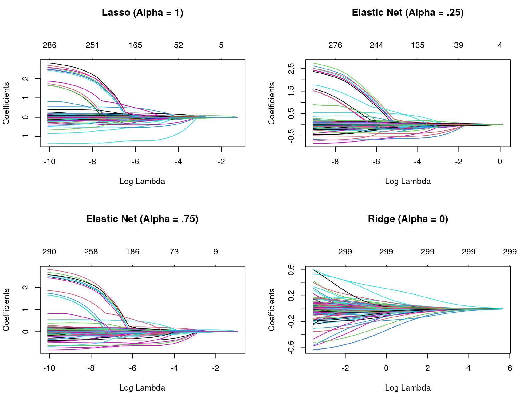
So far we’ve implemented a pure ridge and pure lasso model. However, we can implement an elastic net the same way as the ridge and lasso models, by adjusting the alpha parameter.

lasso    <- glmnet(X, Y, alpha = 1.0) 
elastic1 <- glmnet(X, Y, alpha = 0.25) 
elastic2 <- glmnet(X, Y, alpha = 0.75) 
ridge    <- glmnet(X, Y, alpha = 0.0)

par(mfrow = c(2, 2), mar = c(6, 4, 6, 2) + 0.1)
plot(lasso, xvar = "lambda", main = "Lasso (Alpha = 1)\n\n\n")
plot(elastic1, xvar = "lambda", main = "Elastic Net (Alpha = .25)\n\n\n")
plot(elastic2, xvar = "lambda", main = "Elastic Net (Alpha = .75)\n\n\n")
plot(ridge, xvar = "lambda", main = "Ridge (Alpha = 0)\n\n\n")

Figure 6.1: Coefficients for various penalty parameters.

Often, the optimal model contains an alpha somewhere between 0–1, thus we want to tune both the λ and the alpha parameters.

# for reproducibility
set.seed(123)

# grid search across 
cv_glmnet <- train(
  x = X,
  y = Y,
  method = "glmnet",
  preProc = c("zv", "center", "scale"),
  trControl = trainControl(method = "cv", number = 10),
  tuneLength = 10
)

# model with lowest RMSE
cv_glmnet$bestTune

##   alpha     lambda
## 7   0.1 0.02006835

# plot cross-validated RMSE
ggplot(cv_glmnet) + 
     theme_minimal()

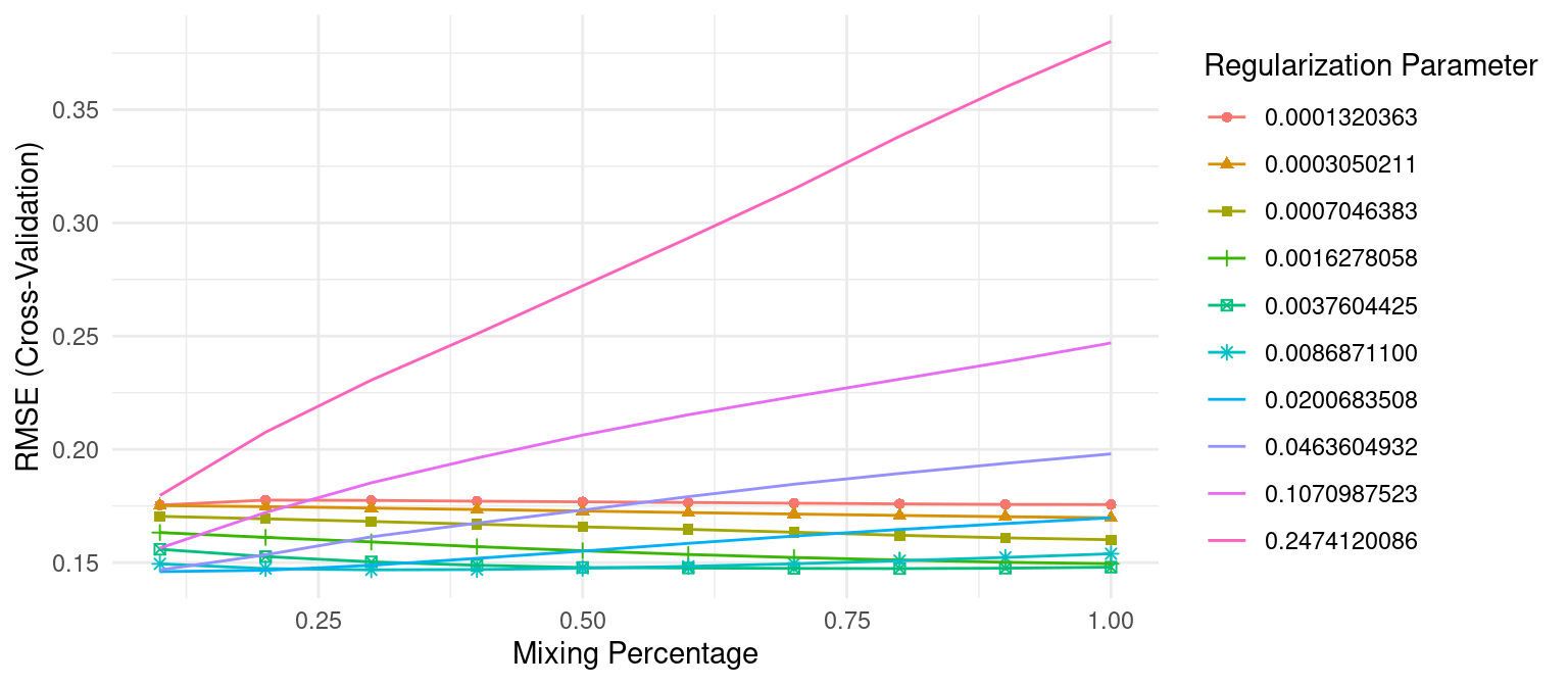
Figure 6.2: The 10-fold cross valdation RMSE across 10 alpha values (x-axis) and 10 lambda values (line color).

The above snippet of code shows that the model that minimized RMSE used an alpha of 0.1 and λ of 0.02. The minimum RMSE of 0.1277585 (MSE=0.1277585^2 = 0.01632223) slightly improves upon the full ridge and lasso models produced earlier.

So how does this compare to our previous best model for the Ames data set? Keep in mind that for this chapter we log transformed the response variable (Sale_Price).

# predict sales price on training data
pred <- predict(cv_glmnet, X)

# compute RMSE of transformed predicted
RMSE(exp(pred), exp(Y))

## [1] 23281.59

Compared with the PLS model’s RMSE of $25,460. the optimized regularization regression model performs better.