One-hot & dummy encoding

Many models require that all predictor variables be numeric. Consequently, we need to intelligently transform any categorical variables into numeric representations so that these algorithms can compute. Some packages automate this process (e.g., h2o and caret) while others do not (e.g., glmnet and keras). There are many ways to recode categorical variables as numeric (e.g., one-hot, ordinal, binary, sum, and Helmert).

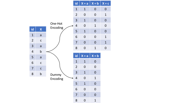
The most common is referred to as one-hot encoding, where we transpose our categorical variables so that each level of the feature is represented as a boolean value.

Figure 3.9: Eight observations containing a categorical feature X and the difference in how one-hot and dummy encoding transforms this feature.

We can one-hot or dummy encode with the same function (step_dummy()). By default, step_dummy() will create a full rank encoding but you can change this by setting one_hot = TRUE.

Comment: Since one-hot encoding adds new features it can significantly increase the dimensionality of our data.

Label encoding

Label encoding is a pure numeric conversion of the levels of a categorical variable. If a categorical variable is a factor and it has pre-specified levels then the numeric conversion will be in level order. If no levels are specified, the encoding will be based on alphabetical order.

ames_train %>% 
     count(MS_SubClass)

## # A tibble: 15 × 2
##    MS_SubClass                                   n
##    <fct>                                     <int>
##  1 One_Story_1946_and_Newer_All_Styles         756
##  2 One_Story_1945_and_Older                     94
##  3 One_Story_with_Finished_Attic_All_Ages        4
##  4 One_and_Half_Story_Unfinished_All_Ages       13
##  5 One_and_Half_Story_Finished_All_Ages        203
##  6 Two_Story_1946_and_Newer                    404
##  7 Two_Story_1945_and_Older                     90
##  8 Two_and_Half_Story_All_Ages                  14
##  9 Split_or_Multilevel                          85
## 10 Split_Foyer                                  37
## 11 Duplex_All_Styles_and_Ages                   76
## 12 One_Story_PUD_1946_and_Newer                132
## 13 Two_Story_PUD_1946_and_Newer                 86
## 14 PUD_Multilevel_Split_Level_Foyer             12
## 15 Two_Family_conversion_All_Styles_and_Ages    43

# Label encoded
recipe(Sale_Price ~ ., data = ames_train) %>%
     step_integer(MS_SubClass) %>%
     prep(ames_train) %>%
     bake(ames_train) %>%
     count(MS_SubClass)

## # A tibble: 15 × 2
##    MS_SubClass     n
##          <int> <int>
##  1           1   756
##  2           2    94
##  3           3     4
##  4           4    13
##  5           5   203
##  6           6   404
##  7           7    90
##  8           8    14
##  9           9    85
## 10          10    37
## 11          11    76
## 12          12   132
## 13          14    86
## 14          15    12
## 15          16    43

We should be careful with label encoding unordered categorical features because most models will treat them as ordered numeric features. If a categorical feature is naturally ordered then label encoding is a natural choice (most commonly referred to as ordinal encoding). For example, the various quality features in the Ames housing data are ordinal in nature (ranging from Very_Poor to Very_Excellent).

ames_train %>% 
     select(contains('Qual'))

## # A tibble: 2,049 × 6
##    Overall_Qual  Exter_Qual Bsmt_Qual   Low_Qual_Fin_SF Kitchen_Qual Garage_Qual
##    <fct>         <fct>      <fct>                 <int> <fct>        <fct>      
##  1 Average       Typical    Typical                   0 Typical      Typical    
##  2 Above_Average Typical    Typical                   0 Typical      Typical    
##  3 Good          Typical    Good                      0 Typical      Typical    
##  4 Above_Average Typical    Good                      0 Typical      Typical    
##  5 Average       Typical    Typical                   0 Typical      Typical    
##  6 Above_Average Typical    No_Basement               0 Typical      Typical    
##  7 Average       Typical    Typical                   0 Typical      Typical    
##  8 Average       Typical    Typical                   0 Typical      Typical    
##  9 Average       Typical    Typical                   0 Typical      No_Garage  
## 10 Average       Typical    Typical                   0 Typical      Typical    
## # ℹ 2,039 more rows

Ordinal encoding these features provides a natural and intuitive interpretation and can logically be applied to all models.

ames_train %>% 
     count(Overall_Qual)

## # A tibble: 10 × 2
##    Overall_Qual       n
##    <fct>          <int>
##  1 Very_Poor          3
##  2 Poor               9
##  3 Fair              33
##  4 Below_Average    147
##  5 Average          580
##  6 Above_Average    521
##  7 Good             408
##  8 Very_Good        242
##  9 Excellent         82
## 10 Very_Excellent    24

# Label encoded
recipe(Sale_Price ~ ., data = ames_train) %>%
     step_integer(Overall_Qual) %>%
     prep(ames_train) %>%
     bake(ames_train) %>%
     count(Overall_Qual)

## # A tibble: 10 × 2
##    Overall_Qual     n
##           <int> <int>
##  1            1     3
##  2            2     9
##  3            3    33
##  4            4   147
##  5            5   580
##  6            6   521
##  7            7   408
##  8            8   242
##  9            9    82
## 10           10    24